Spectral analysis of population cycles

Reading a periodogram to find ecological cycles, why the raw periodogram is noisy, how aliasing turns a fast cycle into a slow one, and why a peak means nothing without a red-noise null.

Some of the most striking patterns in ecology are cycles: lynx and hare on a roughly ten-year rhythm, voles on three to five, insect outbreaks that return like clockwork. The time-domain tools of the previous posts describe how a series depends on its own past. Spectral analysis asks a different question: at what rhythm does the series vary? It decomposes the variance of a series into contributions from cycles of every frequency, and the periodogram is the estimate. Used carelessly it is a machine for inventing cycles, so this post is built around three cautions that matter more than the method itself: the periodogram is noisy and needs smoothing, undersampling disguises fast cycles as slow ones, and a peak is not a cycle until it beats the right null.

Everything is base stats: spec.pgram and a little algebra for the spectra.

The periodogram, and why it needs smoothing

The periodogram splits the total variance of a series across frequencies from zero to one half, the highest frequency a regularly sampled series can carry. A genuine cycle shows up as a peak at its frequency, the reciprocal of its period. We start with a clean case: a ten-step cycle buried in mild noise.

set.seed(4242)
n <- 200; P_true <- 10; t <- 1:n
y <- 2 * cos(2 * pi * t / P_true) + as.numeric(arima.sim(list(ar = 0.3), n = n, sd = 1))

sp_raw <- spec.pgram(y, taper = 0, detrend = TRUE, log = "no", plot = FALSE)
sp_sm  <- spec.pgram(y, spans = 3, taper = 0.1, detrend = TRUE, log = "no", plot = FALSE)  # Daniell(3)
peak_raw <- 1 / sp_raw$freq[which.max(sp_raw$spec)]
peak_sm  <- 1 / sp_sm$freq[which.max(sp_sm$spec)]
cv_raw <- sd(sp_raw$spec) / mean(sp_raw$spec)
cv_sm  <- sd(sp_sm$spec) / mean(sp_sm$spec)

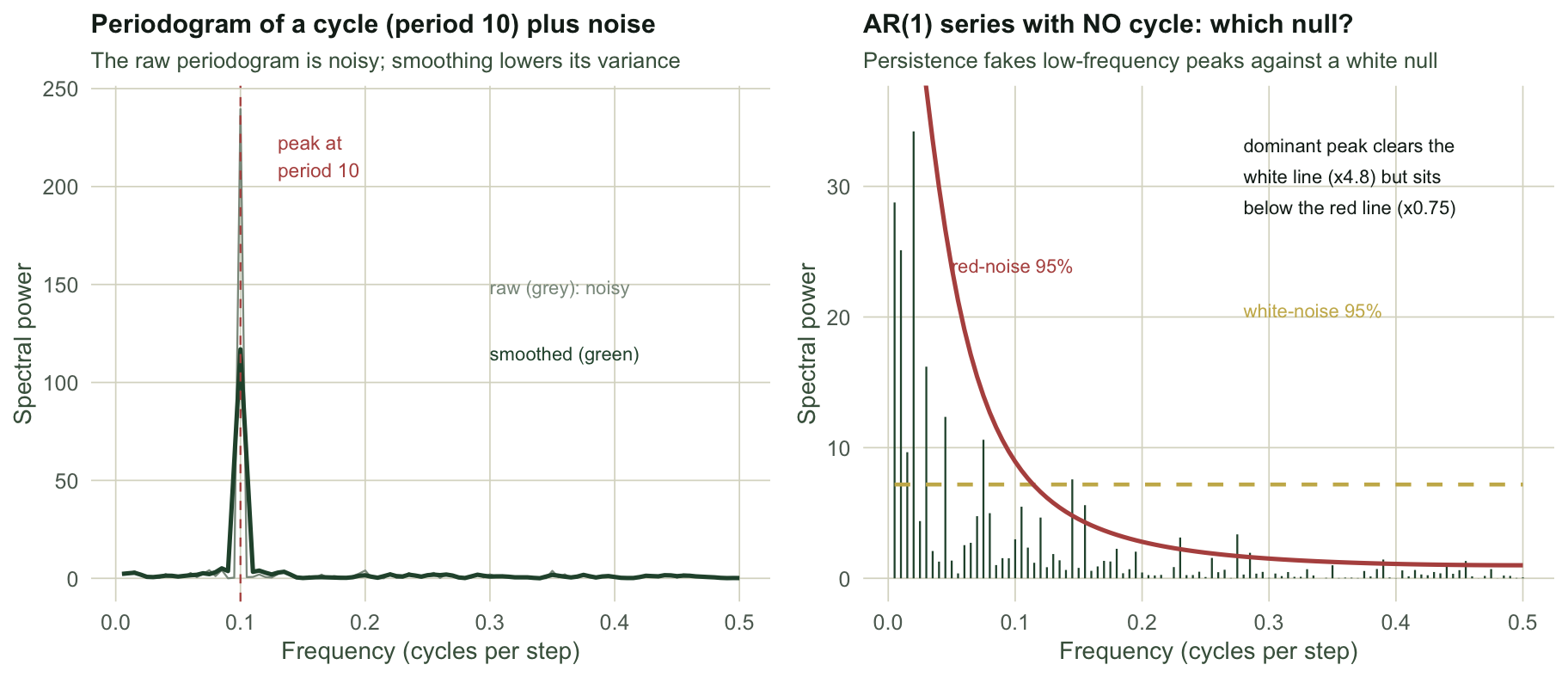
Both the raw and the smoothed periodogram put the peak at a period of 10 steps, recovering the built-in cycle. The problem is everything around the peak. The raw periodogram at each frequency has only two degrees of freedom no matter how long the series, so it never settles down: lengthening the record adds more frequencies but does not make any one estimate less noisy. That is why a raw periodogram looks like grass. Smoothing across neighbouring frequencies, here a short Daniell window, trades a little frequency resolution for a large drop in variance. The coefficient of variation of the ordinates falls from 6.8 in the raw periodogram to 4.0 after smoothing, and the peak stands out far more cleanly against a calmer background.

Aliasing: fast cycles wearing slow disguises

The upper frequency limit, one half of a cycle per sampling interval, is the Nyquist frequency, and it is unforgiving. Any real variation faster than that does not vanish; it folds back down and reappears at a lower frequency, indistinguishable from a genuine slow cycle. This is aliasing, and for ecologists who sample monthly, annually, or whenever the field season allows, it is a live danger. A process with a fast intrinsic rhythm, sampled too coarsely, will show a periodogram peak at a period that simply does not exist.

set.seed(303)
Nf <- 600; P_fast <- 3                         # a period-3 cycle in fine steps
xf <- 1.5 * cos(2 * pi * (1:Nf) / P_fast) + rnorm(Nf, 0, 0.4)
m <- 2                                         # keep every 2nd point (undersample)
xc <- xf[seq(1, Nf, by = m)]

spf <- spec.pgram(xf, taper = 0, detrend = TRUE, log = "no", plot = FALSE)
spc <- spec.pgram(xc, taper = 0, detrend = TRUE, log = "no", plot = FALSE)
peak_fine   <- 1 / spf$freq[which.max(spf$spec)]              # in fine steps
peak_coarse <- 1 / (spc$freq[which.max(spc$spec)] / m)        # back in original steps
nyq_coarse  <- 1 / (2 * m)

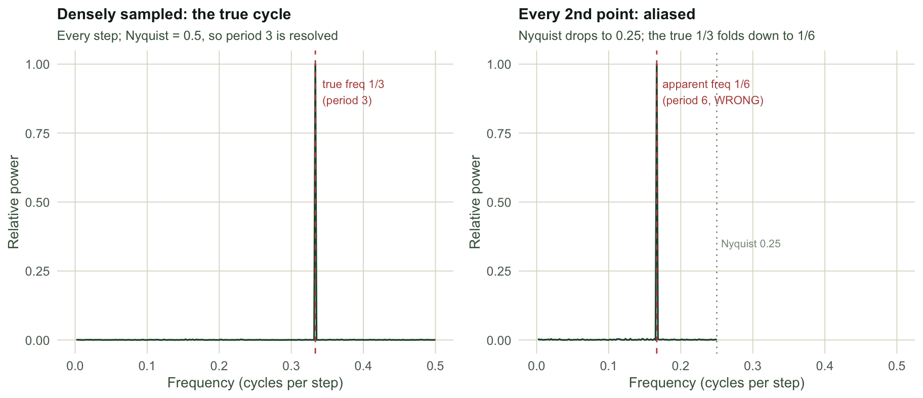
Sampled at every step, the periodogram correctly places the peak at a period of 3 steps: the true frequency of one third sits below the Nyquist limit of one half, so it is resolved. Keep only every second observation and the Nyquist frequency drops to 0.25 cycles per step. The true frequency of one third now lies above that ceiling, folds back, and the periodogram of the thinned series shows its peak at a period of 6 steps, exactly twice the truth. Nothing in the coarse series flags the error: the aliased peak looks like a perfectly respectable cycle. The only defences are sampling fast enough to place expected rhythms below Nyquist, and treating any near-Nyquist peak with suspicion.

Figure 1: Aliasing. Sampled every step (left), the period-3 cycle appears at frequency one third, below the Nyquist limit. Sampled every second step (right), the Nyquist limit drops to 0.25 and the true frequency folds down to one sixth, a phantom period-6 cycle.

A peak is not a cycle: the red-noise null

The deepest trap is the most tempting. Ecological series are rarely white noise; they are persistent, with this year resembling last. A persistent series has a red spectrum, more power at low frequencies simply because of the carry-over, and that low-frequency power piles up into periodogram peaks that look like long cycles but are nothing more than autocorrelation. Testing a peak against a white-noise null, a flat threshold, will therefore manufacture cycles from ordinary persistence. The correct baseline is a red-noise null: the spectrum expected from a fitted autoregressive process with no periodic component.

set.seed(202)
phi <- 0.75
r <- as.numeric(arima.sim(list(ar = phi), n = n, sd = 1))    # persistent, NO cycle
spa <- spec.pgram(r, taper = 0, detrend = TRUE, log = "no", plot = FALSE)
f <- spa$freq; Pgram <- spa$spec

fit1 <- arima(r, order = c(1, 0, 0)); ph <- coef(fit1)["ar1"]; s2 <- fit1$sigma2
ar_spec <- s2 / (1 - 2 * ph * cos(2 * pi * f) + ph^2)         # AR(1) spectral density
ar_spec <- ar_spec * (mean(Pgram) / mean(ar_spec))            # match average power
white_thr <- mean(Pgram) * qchisq(0.95, 2) / 2                # flat 95% threshold
red_thr   <- ar_spec * qchisq(0.95, 2) / 2                    # rising 95% threshold

imax <- which.max(Pgram)
lo <- f < 0.1
n_white_lo <- sum(Pgram[lo] > white_thr)
n_red_lo   <- sum(Pgram[lo] > red_thr[lo])

The series has no cycle at all, only strong persistence, yet its periodogram is dominated by a low-frequency peak at a period of 50 steps. That peak stands 4.8 times above the white-noise threshold, so a white-null test would announce a long cycle with apparent confidence. Against the red-noise null it is a different story: the threshold rises towards low frequency exactly where the persistence puts its power, and the peak reaches only 0.75 of it, correctly judged no cycle. Across the whole low-frequency band, 7 ordinates clear the white-noise line while 0 clear the red-noise line. The lesson generalises past AR(1): the pseudo-cycles of an AR(2) process, like the one built in the previous post, also produce a real spectral peak, and telling a driven cycle from internally generated quasi-periodicity is genuinely hard. The honest workflow states the null before reading the peak.

Figure 2: Left: a cycle plus noise, raw periodogram (grey) against a smoothed one (green). Right: an AR(1) series with no cycle; low-frequency peaks clear the white-noise threshold (gold, flat) but not the red-noise threshold (rust, rising), which expects that low-frequency power.

What to carry away

The periodogram is a sharp tool with three blunt edges. It is inconsistent, so read a smoothed version and never trust the height of a single raw ordinate. It is bounded by the Nyquist frequency, so a cycle faster than twice your sampling interval will lie about its period, and the only cure is sampling design, not analysis. And it sits on top of whatever autocorrelation the series already has, so a peak is evidence of a cycle only when it clears a red-noise null built from a fitted autoregressive spectrum, not the flat white-noise line. A genuine ecological cycle can survive all three tests; the reason spectral claims in ecology are held to a high bar is that so many candidate peaks do not. The checking post brings these frequency-domain diagnostics together with the time-domain ones from across the series.

Related tutorials

• Fitting ARIMA models to ecological time series
• Temporal autocorrelation and effective sample size
• Checking a time series model
• Detecting density dependence

References

• Bloomfield 2000 Fourier Analysis of Time Series: An Introduction, 2nd ed, Wiley, ISBN 978-0-471-88948-9
• Cazelles, Chavez, Berteaux, Menard, Vik, Jenouvrier & Stenseth 2008 Oecologia 156(2):287-304 (10.1007/s00442-008-0993-2)
• Platt & Denman 1975 Annual Review of Ecology and Systematics 6:189-210 (10.1146/annurev.es.06.110175.001201)
• Shumway & Stoffer 2017 Time Series Analysis and Its Applications, 4th ed, Springer, ISBN 978-3-319-52451-1