Fitting ARIMA models to ecological time series

Identifying an autoregressive-moving-average model from the ACF and PACF, fitting it with base R arima(), forecasting with honest prediction intervals, and the twin traps of over-differencing and plug-in overconfidence.

Once you can read a correlogram, you can build a model for a time series. The autoregressive integrated moving-average family, ARIMA, is the standard toolkit for describing and forecasting a single series: a population index, a monthly temperature record, a phenological signal. The Box-Jenkins approach turns the autocorrelation and partial autocorrelation functions from the previous post into a recipe: read the correlograms to pick the model, fit it, then check the forecast. This post walks through identification, fitting with base R arima(), and forecasting, and it is honest about the two places the workflow misleads: over-differencing manufactures structure that was never there, and the tidy prediction interval assumes the model and its parameters are exactly right.

Everything is base stats: arima, predict, diff, AIC.

Reading the correlograms to identify a model

Many ecological series oscillate. A second-order autoregressive process, AR(2), is the simplest model that produces a pseudo-cycle: with the right coefficients its own dynamics generate quasi-periodic swings without any external forcing, which is exactly how predator-prey and rodent populations are often described. We simulate such a series and read its signature.

set.seed(4241)
phi1 <- 1.2; phi2 <- -0.6; n <- 160
y <- as.numeric(arima.sim(list(ar = c(phi1, phi2)), n = n, sd = 1))

pseudo_T <- 2 * pi / acos(phi1 / (2 * sqrt(-phi2)))   # induced pseudo-period
pac <- as.numeric(pacf(y, lag.max = 12, plot = FALSE)$acf)

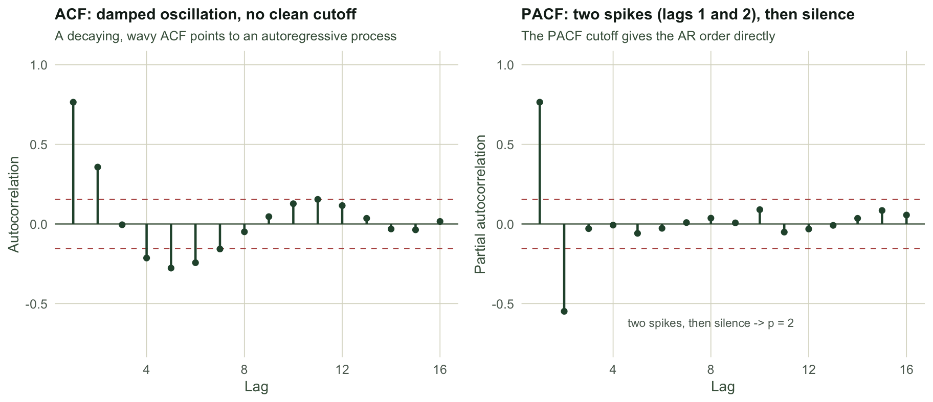
The two coefficients induce a pseudo-cycle of about 9.2 steps, visible as the damped wave in the ACF below. Identification is a division of labour between the two correlograms. An autoregressive process of order p has a PACF that spikes at lags 1 to p and then falls silent, while its ACF decays gradually. A moving-average process of order q shows the mirror image: the ACF cuts off after lag q and the PACF trails away. For our series the PACF has clear spikes at lag 1 (0.765) and lag 2 (-0.549) and nothing beyond (lag 3 is -0.029). That reads directly as p = 2, with no moving-average term needed. The series is stationary, so no differencing: an ARIMA(2, 0, 0).

Figure 1: Identifying an AR(2) model. The ACF is a damped oscillation; the PACF spikes at lags 1 and 2 then falls within the band, giving the order p = 2 directly.

Fitting and comparing orders

With the order chosen, arima() fits the coefficients by maximum likelihood. It reports each coefficient with a standard error, which is where honest inference begins.

fit <- arima(y, order = c(2, 0, 0), include.mean = TRUE)
b <- coef(fit); se <- sqrt(diag(fit$var.coef))

The fit recovers the generating coefficients well: phi1 is estimated at 1.203 (true 1.2) and phi2 at -0.563 (true -0.6), each with a standard error of about 0.065. Reading the correlograms is a starting point, not a verdict, so it is worth comparing a few nearby orders by AIC rather than trusting the eye alone.

orders <- list("AR(1)" = c(1,0,0), "AR(2)" = c(2,0,0), "AR(3)" = c(3,0,0),
               "ARMA(1,1)" = c(1,0,1), "ARMA(2,1)" = c(2,0,1))
aics <- sapply(orders, function(o) AIC(arima(y, order = o, include.mean = TRUE)))
d_aic <- round(aics - min(aics), 1)

The AIC agrees with the correlograms. AR(2) has the lowest value; AR(1) is 58.5 higher (it cannot make the oscillation), while AR(3) and ARMA(2,1) sit 1.8 above it, meaning the extra parameter buys nothing. ARMA(1,1) is 20 higher. The simplest model that captures the dynamics wins, which is the parsimony the whole approach is built on.

Differencing, and the trap of over-differencing

When a series wanders without settling around a fixed level, a trend or a unit root, it is not stationary and the models above do not apply directly. Differencing, replacing the series by its step-to-step changes, usually restores stationarity: that is the “I” in ARIMA, the middle order d. The temptation is to difference routinely, but differencing a series that was already stationary does real harm. It injects a moving-average term that was never in the data.

set.seed(4241)
z <- as.numeric(arima.sim(list(ar = 0.5), n = 160))   # stationary: the correct d is 0
dz <- diff(z)                                          # differenced anyway
od <- arima(dz, order = c(0, 0, 1), include.mean = FALSE)
acf_dz <- as.numeric(acf(dz, lag.max = 3, plot = FALSE)$acf)

The original series is a plain stationary AR(1) that needs no differencing. Difference it anyway and the changes carry a strong negative lag-1 autocorrelation (-0.332), and a moving-average fit picks up an artificial coefficient of -0.521, heading towards the tell-tale value of minus one. A negative moving-average term near minus one in the differences is the classic footprint of over-differencing: the cure for a problem the series did not have. The lesson is to difference only when the series is genuinely non-stationary, and to check that the differences do not show this negative spike.

Forecasting, and how honest the interval is

Forecasting is where a fitted model earns its keep, and where overconfidence hides. predict() extends the series and returns a standard error at each horizon, from which we build a 95% band. We fit on the first part of the series and forecast the held-out tail.

ntr <- 120; h <- 24
ytr <- y[1:ntr]; yte <- y[(ntr + 1):(ntr + h)]
fit_tr <- arima(ytr, order = c(2, 0, 0))
pr <- predict(fit_tr, n.ahead = h)
pred <- as.numeric(pr$pred); lo <- pred - 1.96 * pr$se; hi <- pred + 1.96 * pr$se
in_band <- sum(yte >= lo & yte <= hi)

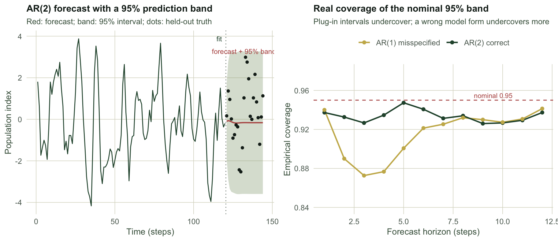
The forecast oscillates for a few steps, then the pseudo-cycle damps and the series is drawn back towards its long-run mean, with the band widening to a stable width as the horizon grows. In this run all 24 of the 24 held-out points fall inside the 95% band. One clean forecast, though, proves little. The stated interval rests on two assumptions: that AR(2) is the right form, and that the estimated coefficients equal the true ones. predict.Arima treats the fitted parameters as if they were known exactly, a plug-in interval that ignores the uncertainty in those estimates. To see the cost, we repeat the fit-and-forecast over many independent series and record how often the nominal 95% band actually contains the truth, using a modest series length where estimation error bites.

ntr2 <- 90; H <- 12; B <- 1500
cov2 <- cov1 <- matrix(NA_real_, B, H)
set.seed(4243)
for (bb in seq_len(B)) {
  s <- as.numeric(arima.sim(list(ar = c(phi1, phi2)), n = ntr2 + H, sd = 1))
  tr <- s[1:ntr2]; te <- s[(ntr2 + 1):(ntr2 + H)]
  f2 <- tryCatch(arima(tr, order = c(2, 0, 0)), error = function(e) NULL)  # correct
  f1 <- tryCatch(arima(tr, order = c(1, 0, 0)), error = function(e) NULL)  # misspecified
  if (!is.null(f2)) { p <- predict(f2, n.ahead = H); cov2[bb, ] <- as.numeric(te >= p$pred - 1.96 * p$se & te <= p$pred + 1.96 * p$se) }
  if (!is.null(f1)) { p <- predict(f1, n.ahead = H); cov1[bb, ] <- as.numeric(te >= p$pred - 1.96 * p$se & te <= p$pred + 1.96 * p$se) }
}
e2 <- colMeans(cov2, na.rm = TRUE); e1 <- colMeans(cov1, na.rm = TRUE)

Even with the correct AR(2) form, the nominal 95% band covers the truth about 93% of the time on average, a little short because the plug-in interval treats estimated parameters as fixed. Fit the wrong form, an AR(1) that cannot represent the oscillation, and coverage falls further to about 92%, and it fails worst at the mid-range horizons where the missing cycle matters most (87% at three steps). The shape of the shortfall is diagnostic: an interval that undercovers at exactly the horizons a missing dynamic would bite is telling you the model form, not the arithmetic, is wrong.

Don't know how to automatically pick scale for object of type <ts>. Defaulting
to continuous.
Don't know how to automatically pick scale for object of type <ts>. Defaulting
to continuous.

Figure 2: Left: an AR(2) forecast with its 95% band; the pseudo-cycle damps towards the mean and the held-out points fall inside. Right: the true coverage of the nominal 95% band. Even the correct model undercovers slightly; a misspecified AR(1) undercovers more, worst at the horizons where the cycle matters.

What to carry away

The Box-Jenkins loop is a genuine workflow: read the ACF and PACF to propose an order, confirm it against a small set of alternatives by AIC, fit with arima(), then forecast. Two cautions keep it honest. Difference only a series that truly needs it; a negative moving-average spike near minus one in the differences means you have over-differenced and should step back to a lower d. And treat the forecast band as a floor on the uncertainty, not the whole of it: the plug-in interval assumes the model and its parameters are exactly right, so its real coverage is a little below nominal even in the best case and can fall well short when the model form is wrong. An interval that undercovers is not a rounding error; it is the model telling you something. The checking post makes that diagnosis its subject. The next post takes the pseudo-cycle we built here and asks the frequency-domain question: is the periodicity real, and at what period?

Related tutorials

• Temporal autocorrelation and effective sample size
• Spectral analysis of population cycles
• Checking a time series model
• Detecting density dependence

References

• Box, Jenkins, Reinsel & Ljung 2015 Time Series Analysis: Forecasting and Control, 5th ed, Wiley, ISBN 978-1-118-67502-1
• Hyndman & Athanasopoulos 2021 Forecasting: Principles and Practice, 3rd ed, OTexts, ISBN 978-0-9875071-3-6
• Ives, Abbott & Ziebarth 2010 Ecology 91(3):858-871 (10.1890/09-0442.1)
• Shumway & Stoffer 2017 Time Series Analysis and Its Applications, 4th ed, Springer, ISBN 978-3-319-52451-1