---
title: "Detecting density dependence in R"
description: "Fitting a Gompertz model to a population time series in R, why the ordinary regression test for density dependence over-rejects, and the bootstrap fix."
date: "2026-05-14 14:00"
categories: [R, population dynamics, time series, density dependence, ecology tutorial]
image: thumbnail.png
image-alt: "Scatter of per-capita growth against log abundance for a density-dependent series and a random walk, with fitted regression lines."
date-modified: "2026-09-27"
---
*Corrected 27 September 2026: the post said the bootstrap test never assumes a distribution; it avoids a theoretical reference distribution for the statistic but still assumes normal process noise, which the text now says.*
Density dependence is the idea that per-capita growth slows as a population gets crowded. Given a single time series of counts, a natural question is whether the data carry any signal of it at all, or whether the ups and downs are just density-independent drift. The problem is that the obvious test for this signal is badly biased, and it declares density dependence far too often. This post fits the standard Gompertz model to a count series in base R, shows why the ordinary regression test fails, and replaces it with the parametric bootstrap test of Dennis and Taper.
## The Gompertz model on the log scale
Write $X_t = \log N_t$ for the log abundance in year $t$. The discrete Gompertz model is a first-order autoregression on that log scale:
$$X_{t+1} = a + b\,X_t + \varepsilon_t, \qquad \varepsilon_t \sim \mathrm{Normal}(0, \sigma^2).$$
The slope $b$ is the whole story. When $b = 1$ the model is a random walk with drift: shocks never fade, the population wanders without any pull back towards a typical size, and growth does not depend on density. When $b < 1$ there is density dependence: a population above its equilibrium tends to shrink, one below it tends to grow, and the log abundance is pulled towards a stationary mean $X^{*} = a / (1 - b)$. The quantity $1 - b$ is the return rate, the fraction of a deviation that is removed in one year. So the entire test for density dependence is a test of $b < 1$ against the density-independent null $b = 1$.
```{r}
#| label: setup
#| code-fold: true
#| code-summary: "Setup: packages, colours and plot theme"
#| results: hide
#| message: false
#| warning: false
suppressPackageStartupMessages({library(ggplot2); library(dplyr)})
ink<-"#16241d"; body<-"#2c3a31"; forest<-"#275139"; gold<-"#c9b458"
paper<-"#f5f4ee"; line<-"#dad9ca"; faint<-"#5d6b61"; aban<-"#b5534e"
theme_te <- function(){
  theme_minimal(base_size=12)+
  theme(plot.background=element_rect(fill=paper,colour=NA),
        panel.background=element_rect(fill=paper,colour=NA),
        panel.grid.minor=element_blank(),
        panel.grid.major=element_line(colour=line,linewidth=.3),
        axis.title=element_text(colour=ink), axis.text=element_text(colour=faint),
        plot.title=element_text(colour=ink,size=12,face="bold"),
        strip.text=element_text(colour=ink,face="bold"),
        legend.position="bottom", legend.title=element_text(colour=ink),
        legend.text=element_text(colour=body))
}
```
The likelihood is Gaussian and the fit is nothing more than a linear regression of $X_{t+1}$ on $X_t$, so ordinary least squares gives the maximum likelihood estimates of $a$ and $b$ directly. Two small helper functions do the work: one fits the autoregression and also returns the likelihood ratio against the null $b = 1$, the other simulates a series.
```{r}
#| label: helpers
fit_ar1 <- function(x){
  n <- length(x); x0 <- x[-n]; x1 <- x[-1]; m <- n-1; xb <- mean(x0)
  Sxx <- sum((x0-xb)^2)
  b <- sum((x0-xb)*(x1-mean(x1)))/Sxx
  a <- mean(x1) - b*xb
  r <- x1 - (a + b*x0); s2 <- sum(r^2)/m
  se_b <- sqrt((sum(r^2)/(m-2))/Sxx)
  d <- x1 - x0; a0 <- mean(d); s20 <- mean((d-a0)^2)
  LR <- m*(log(s20) - log(s2))       # 2*(logLik_full - logLik_null), constants cancel
  list(a=a,b=b,s2=s2,se_b=se_b,m=m,LR=LR,a0=a0,s20=s20,grow=d,x0=x0)
}
sim_gompertz <- function(T,a,b,s,x1){ x<-numeric(T); x[1]<-x1
  for(t in 1:(T-1)) x[t+1] <- a + b*x[t] + rnorm(1,0,s); x }
```
## Two series that look alike
To see the problem, simulate two series of the same length. The first has genuine density dependence ($b = 0.60$, equilibrium at $N^{*} = 140$); the second is a pure driftless random walk ($b = 1$), the density-independent null. Both run for 35 years with the same noise level.
```{r}
#| label: simulate
Tlen<-35; Nstar<-140; Xstar<-log(Nstar); b_dd<-0.60; s_dd<-0.20; a_dd<-(1-b_dd)*Xstar

set.seed(932)
Xdd <- sim_gompertz(Tlen, a_dd, b_dd, s_dd, x1=log(70))   # density dependent

set.seed(3075)
Xrw <- sim_gompertz(Tlen, 0, 1, 0.20, x1=Xstar)          # random walk (b = 1)
```
Fitting the Gompertz model to each gives the slope estimate and its ordinary standard error.
```{r}
#| label: fits
fdd <- fit_ar1(Xdd)
frw <- fit_ar1(Xrw)
naive_p <- function(f) pt((f$b-1)/f$se_b, df=f$m-2)      # one-sided t test of b < 1

round(c(dd_b=fdd$b, dd_se=fdd$se_b, dd_Nstar=exp(fdd$a/(1-fdd$b)),
        rw_b=frw$b, rw_se=frw$se_b), 3)
round(c(dd_naive_p=naive_p(fdd), rw_naive_p=naive_p(frw)), 4)
```
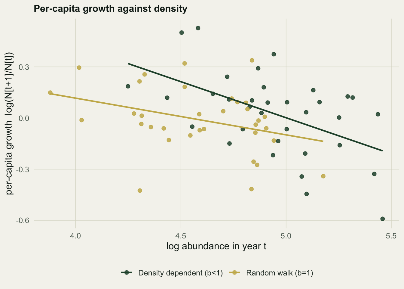
For the density-dependent series the slope comes out at $\hat b = 0.58$ with an implied equilibrium of $\hat N^{*} = 149$, close to the truth. For the random walk the slope is $\hat b = 0.79$, comfortably below one, and a one-sided $t$ test of $b < 1$ returns $p = 0.023$. Taken at face value that $p$ value says the random walk shows density dependence. It does not: the series was generated with $b = 1$ and no density dependence at all. The plot of per-capita growth against density tells the same misleading story, with a downward slope on both series.
```{r}
#| label: fig-growth
#| fig-cap: "Per-capita growth against log abundance. The density-dependent series slopes down as expected, but the random walk also appears to slope down, because the slope estimate is biased."
#| fig-alt: "Scatter of per-capita growth against log abundance for two series, density dependent in green and random walk in gold, each with a downward fitted line."
gd <- rbind(
  data.frame(x=fdd$x0, r=fdd$grow, series="Density dependent (b<1)"),
  data.frame(x=frw$x0, r=frw$grow, series="Random walk (b=1)"))
ggplot(gd, aes(x, r, colour=series))+
  geom_hline(yintercept=0, colour=faint, linewidth=.3)+
  geom_point(size=1.9, alpha=.85)+
  geom_smooth(method="lm", se=FALSE, linewidth=.9, formula=y~x)+
  scale_colour_manual(values=c("Density dependent (b<1)"=forest,"Random walk (b=1)"=gold))+
  labs(x="log abundance in year t", y="per-capita growth  log(N[t+1]/N[t])",
       colour=NULL, title="Per-capita growth against density")+
  theme_te()
```
## Why the ordinary test misleads
The failure has a clean explanation. When the true slope sits at or near one, the least squares estimate of an autoregressive coefficient is biased downwards: the fitted $\hat b$ is systematically smaller than the value that generated the data. On top of that, the sampling distribution of the test statistic under the null is not the $t$ distribution at all; it is the non-standard unit-root distribution studied by Dickey and Fuller. Feeding a biased estimate into the wrong reference distribution is a recipe for false alarms.
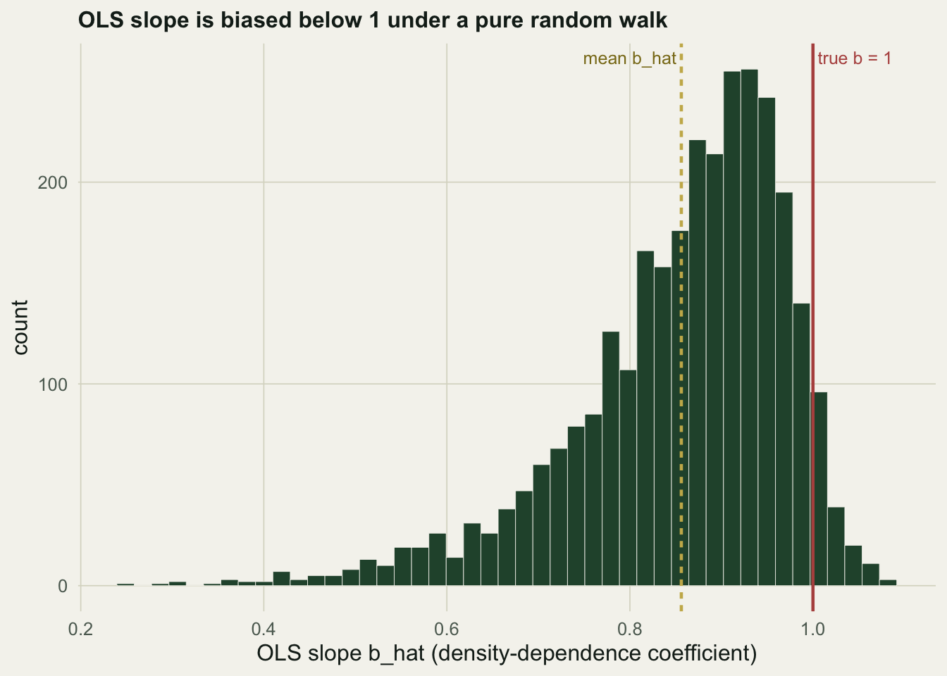
The size of the bias is easy to measure. Generate three thousand random walks, fit the Gompertz slope to each, and look at where the estimates land.
```{r}
#| label: bias-sim
set.seed(2468); M<-3000; bh<-numeric(M); rej<-logical(M)
for(i in 1:M){
  Xr <- sim_gompertz(Tlen, 0, 1, 0.20, x1=Xstar)
  f <- fit_ar1(Xr); bh[i] <- f$b; rej[i] <- naive_p(f) < 0.05
}
round(c(mean_bhat=mean(bh), bias=1-mean(bh), median=median(bh), naive_reject=mean(rej)), 3)
```
Under a true random walk the average slope is $0.86$, not $1$: a downward bias of about $0.14$. The consequence is severe. The one-sided $t$ test, run at a nominal five per cent level, rejects the density-independent null in $42\%$ of these series. A test that is supposed to make a false claim of density dependence one time in twenty makes it two times in five.
```{r}
#| label: fig-bias
#| fig-cap: "Sampling distribution of the ordinary least squares slope under a true random walk. The estimates pile up below the true value of one, which is why the naive test finds density dependence so often."
#| fig-alt: "Histogram of fitted slope estimates from three thousand random walks, centred near 0.86, with a red line at the true value one and a dashed line at the mean."
dfb <- data.frame(b=bh)
ggplot(dfb, aes(b))+
  geom_histogram(bins=45, fill=forest, colour=paper, linewidth=.15)+
  geom_vline(xintercept=1, colour=aban, linewidth=.8)+
  geom_vline(xintercept=mean(bh), colour=gold, linewidth=.8, linetype="22")+
  annotate("text", x=1, y=Inf, label=" true b = 1", hjust=0, vjust=1.6, colour=aban, size=3.3)+
  annotate("text", x=mean(bh), y=Inf, label="mean b_hat ", hjust=1, vjust=1.6, colour="#8a7a1e", size=3.3)+
  labs(x="OLS slope b_hat (density-dependence coefficient)", y="count",
       title="OLS slope is biased below 1 under a pure random walk")+
  theme_te()
```
## The parametric bootstrap test
The fix from Dennis and Taper is to stop trusting the theoretical reference distribution and build the correct one by simulation. Fit the density-independent null to the observed series, giving a drift and a noise variance. Simulate many random walks from that fitted null, and for each one compute the same likelihood ratio statistic that compares the free Gompertz fit against $b = 1$. The collection of simulated statistics is the null distribution for this particular series and length. The bootstrap $p$ value is the fraction of simulated statistics that reach or exceed the one observed.
```{r}
#| label: pblr
pblr <- function(x, B=1999){
  f <- fit_ar1(x); T <- length(x); LRstar <- numeric(B)
  for(bb in 1:B){
    xs <- numeric(T); xs[1] <- x[1]
    e <- rnorm(T-1, f$a0, sqrt(f$s20))        # simulate under H0: b = 1, drift a0
    for(t in 1:(T-1)) xs[t+1] <- xs[t] + e[t]
    LRstar[bb] <- fit_ar1(xs)$LR
  }
  list(p=(1+sum(LRstar>=f$LR))/(B+1), LRobs=f$LR)
}
set.seed(9321);  pdd <- pblr(Xdd, B=1999)     # density-dependent series
set.seed(30751); prw <- pblr(Xrw, B=1999)     # random-walk series
round(c(dd_LR=pdd$LRobs, dd_pblr=pdd$p, rw_LR=prw$LRobs, rw_pblr=prw$p), 4)
```
Now the two series part company. The density-dependent series has a likelihood ratio of $10.4$ and a bootstrap $p$ value of $0.015$: real density dependence, correctly flagged. The random walk has a likelihood ratio of $4.3$ and a bootstrap $p$ value of $0.24$: no evidence of density dependence, which is the right answer. The naive $t$ test called both series density dependent; the bootstrap test keeps them apart.
The reason the bootstrap works where the $t$ test does not is that it never assumes a theoretical reference distribution for the test statistic. It does still assume normal process noise, because the null series are simulated with Gaussian steps. The same downward bias in $\hat b$ that fooled the naive test is present in every simulated series too, so it cancels out of the comparison. The observed statistic is judged against statistics generated the same way, on the same length of data.
## Does it hold its nominal level?
The final check is calibration: run the bootstrap test on many series that truly have no density dependence, and confirm it rejects about five per cent of the time. Five hundred random walks, each with a small internal bootstrap, are enough to see it.
```{r}
#| label: calib
set.seed(1357); M2<-500; B2<-299; prej<-logical(M2)
for(i in 1:M2){
  Xr <- sim_gompertz(Tlen, 0, 1, 0.20, x1=Xstar)
  f <- fit_ar1(Xr); LRo <- f$LR; LRs <- numeric(B2)
  for(bb in 1:B2){
    xs <- numeric(Tlen); xs[1] <- Xr[1]
    e <- rnorm(Tlen-1, f$a0, sqrt(f$s20))
    for(t in 1:(Tlen-1)) xs[t+1] <- xs[t] + e[t]
    LRs[bb] <- fit_ar1(xs)$LR
  }
  prej[i] <- (1+sum(LRs>=LRo))/(B2+1) < 0.05
}
round(mean(prej), 3)
```
The bootstrap test rejects in about $5\%$ of density-independent series, against the $42\%$ of the naive test. It does what the nominal level promises.
## What the test does and does not tell you
A significant result says there is statistical support for $b < 1$, meaning the data are pulled back towards a typical size rather than wandering freely. It does not identify the mechanism, and it does not measure how strong the regulation is with any precision: over thirty-five years the slope estimate carries a wide confidence interval, and short series often have too little power to detect real density dependence at all, which is the flip side of the false-alarm problem. The Gompertz slope also mixes any observation error into the estimate. Counting error in the abundances biases the slope further below one, so a series measured with noise can appear more density dependent than it is. Separating that observation error from real population fluctuation is the job of the [Gompertz state-space model](../gompertz-state-space-model/), which fits the process and the counting error at the same time.
## References
Dennis B & Taper ML 1994 Ecological Monographs 64(2):205-224 (10.2307/2937041)
Pollard E, Lakhani KH & Rothery P 1987 Ecology 68(6):2046-2055 (10.2307/1939895)
Bulmer MG 1975 Biometrics 31(4):901-911 (10.2307/2529815)
Dickey DA & Fuller WA 1979 Journal of the American Statistical Association 74(366):427-431 (10.1080/01621459.1979.10482531)
## Related tutorials
- [The Gompertz state-space model](../gompertz-state-space-model/)
- [Spatial synchrony and the Moran effect](../spatial-synchrony-and-the-moran-effect/)
- [Community stability from a MAR(1) model](../stability-from-a-mar1-model/)
- [Culls set by this year's count: a causal trap](../culls-set-by-last-years-count/)