Culls set by this year’s count: a causal trap

When each year’s cull is decided from that year’s count, the count is both mediator and confounder. In R: g-computation, IPTW and a population model compared.

A group of neighbouring estates counts its deer every spring, and on each estate the decision to cull that year is taken from that spring’s count: a high count makes a cull likely, a low one makes it unlikely. A cull takes out four animals in ten. After three seasons the management record holds, for every estate, four counts and three yes-or-no decisions, and the group wants one number from it: how much lower is the count after three years of culling every year than after three years of leaving the deer alone?

The record looks made for a regression of the final count on the three cull decisions, with the counts as covariates. The trouble is that the counts are two things at once. The count in the second spring was lowered by the first cull, so it carries part of the effect the group wants to measure; it also drives the second cull, and the abundance it measures drives the final count, so it confounds the second decision. Leave it out and the second decision is confounded. Put it in and the first cull’s effect through it is thrown away. This is treatment-confounder feedback, and it is the problem Robins (1986) wrote the g-formula for; Daniel and colleagues (2013) review the methods that have grown from it. None of what follows is new to causal inference. The post is a demonstration of those results on a management record, with a generator in which the ecology can be switched on and off. Larsen, Meng and Kendall (2019) review causal designs for observational control-impact studies in ecology; a management decision repeated on the readings it has itself changed needs the time-varying form.

The causal posts on this site build the pieces. G-computation and standardisation fits an outcome model and averages its predictions under each treatment level, for one treatment given at one time. Confounding and backdoor adjustment warns that “Conditioning on M holds the mediator fixed and reports only the leftover direct piece”, which is half of the trap here. Propensity scores and IPW weights by the probability of treatment and reminds the reader that “Weighting only works where both groups exist.” Baseline selection and the return to the mean has one selection from one count, and nothing afterwards reads the counts again. The causal posts adjust for confounders measured before a single treatment and warn against conditioning on a mediator; here last year’s cull made this year’s count, and this year’s count sets this year’s cull, so the count is both at once, and the population model most ecologists would fit instead is right only in the linear case and drifts with how different the estates are. That population model is the Gompertz transition of Detecting density dependence in R with the cull added as a covariate.

Two of the numbers below are known before any simulation runs. Adjusting for every count keeps a share of the effect that has a closed form in the linear case, and sequential g-computation recovers the effect when its working models are close to right, which is Robins’s theorem. Neither is a finding. What the simulation measures is everything around them: how the naive regression moves with the spread of estate capacity, how far the population model drifts, when inverse probability weighting breaks down, and how much of any of this a record of a hundred and fifty estates can show.

library(ggplot2)
library(patchwork)

te_paper  <- "#f5f4ee"
te_ink    <- "#16241d"
te_body   <- "#2c3a31"
te_forest <- "#275139"
te_rust   <- "#b5534e"
te_gold   <- "#c9b458"
te_line   <- "#dad9ca"

theme_datasheet <- function() {
  theme_minimal(base_size = 12) +
    theme(plot.background  = element_rect(fill = te_paper, colour = NA),
          panel.background = element_rect(fill = te_paper, colour = NA),
          panel.grid.major = element_line(colour = te_line, linewidth = 0.3),
          panel.grid.minor = element_blank(),
          text             = element_text(colour = te_body),
          plot.title       = element_text(colour = te_ink, face = "bold"),
          plot.subtitle    = element_text(colour = te_body),
          axis.text        = element_text(colour = te_body))
}

Estates, counts and a cull rule

n_dec   <- 3
r_grow  <- 0.5
h_cull  <- 0.4
log_k0  <- log(80)
sd_proc <- 0.25
sd_init <- 0.3
n_big   <- 20000

rule_logit <- function(slope) {
  function(l, u) as.integer(u < plogis(-0.3 + slope * (l - log_k0)))
}
fixed_cull <- function(a) function(l, u) rep(as.integer(a), length(l))

sim_estates <- function(n_est, sd_k, assign, poisson = TRUE) {
  log_k <- rnorm(n_est, log_k0, sd_k)
  log_n <- log_k + rnorm(n_est, 0, sd_init)
  eps   <- matrix(rnorm(n_est * n_dec, 0, sd_proc), n_est)
  u_dec <- matrix(runif(n_est * n_dec), n_est)
  cnt   <- matrix(NA_real_, n_est, n_dec + 1)
  cull  <- matrix(NA_integer_, n_est, n_dec)
  read_count <- function(x) if (poisson) log(rpois(n_est, exp(x)) + 1) else x
  for (tt in 1:n_dec) {
    cnt[, tt]  <- read_count(log_n)
    cull[, tt] <- assign(cnt[, tt], u_dec[, tt])
    log_after  <- log_n + log(1 - h_cull * cull[, tt])
    log_n      <- log_after + r_grow * (1 - exp(log_after - log_k)) + eps[, tt]
  }
  cnt[, n_dec + 1] <- read_count(log_n)
  list(cnt = cnt, cull = cull)
}

as_record <- function(d) {
  data.frame(y  = d$cnt[, 4], l0 = d$cnt[, 1], l1 = d$cnt[, 2], l2 = d$cnt[, 3],
             a0 = d$cull[, 1], a1 = d$cull[, 2], a2 = d$cull[, 3])
}

regime_effect <- function(seed, sd_k, poisson = TRUE, arm1 = fixed_cull(1),
                          arm0 = fixed_cull(0)) {
  set.seed(seed)
  y_1 <- mean(sim_estates(n_big, sd_k, arm1, poisson)$cnt[, n_dec + 1])
  set.seed(seed)
  y_0 <- mean(sim_estates(n_big, sd_k, arm0, poisson)$cnt[, n_dec + 1])
  y_1 - y_0
}

Each estate has a carrying capacity K, drawn on the log scale around 80 animals with standard deviation sd_k, and it starts near that capacity. Every spring the deer are counted with Poisson error, and the analysis works on log(count + 1), which is what the management record holds. The decision to cull is a coin toss whose probability rises with the count: with slope at 1.5, an estate counting 80 culls with probability 0.43 and one counting 160 with probability 0.68. A cull removes a share h_cull = 0.4 of the animals, and the survivors grow by a Ricker step with rate 0.5 towards the estate’s own K, plus process noise. The cull comes before the growth. After three decisions the fourth count is the outcome.

The estimand is the contrast of two fixed regimes over all estates: the mean log final count if every estate culled in all three years, minus the same mean if none ever culled. regime_effect() computes it by running 20000 estates under each regime with the same random numbers, so the only difference between the two arms is the culling. Every estimate below is reported as a ratio to this truth, recomputed for each simulated record from its own seed.

One count, two roles

The graph below draws two of the three decisions, which is enough to show the problem. The first cull, A0, lowers the true abundance N1, which carries its effect forward through N2 to the final count; the count C1 is a reading of that mediator. (The one directed path from A0 that passes through C1 goes on through A1, which each regime fixes, so it is no part of the contrast.) C1 is also the only input to the second cull A1, and its parent N1 drives the final count, so every backdoor path into A1 runs through C1, as in A1 <- C1 <- N1 -> N2 -> C2. A regression that includes C1 closes those paths, and because C1 stands in for N1, it also absorbs part of the effect of A0 that runs through N1, all of it when the counts are exact. No set of counts does one without the other.

node_xy <- data.frame(
  node  = c("K", "N0", "N1", "N2", "C0", "C1", "C2", "A0", "A1"),
  lab   = c("K", "N[0]", "N[1]", "N[2]", "C[0]", "C[1]", "C[2]", "A[0]", "A[1]"),
  x     = c(2, 0, 2, 4, 0, 2, 4, 1, 3),
  y     = c(2.1, 1, 1, 1, 0, 0, 0, -1, -1),
  kind  = c("hidden", "hidden", "hidden", "hidden", "count", "both", "outcome", "cull", "cull"))
edge_df <- data.frame(
  from = c("K", "K", "K", "N0", "N1", "N0", "N1", "N2", "C0", "C1", "A0", "A1"),
  to   = c("N0", "N1", "N2", "N1", "N2", "C0", "C1", "C2", "A0", "A1", "N1", "N2"))
edge_df <- cbind(edge_df,
                 setNames(node_xy[match(edge_df$from, node_xy$node), c("x", "y")], c("x0", "y0")),
                 setNames(node_xy[match(edge_df$to, node_xy$node), c("x", "y")], c("x1", "y1")))
shrink <- 0.24
len    <- sqrt((edge_df$x1 - edge_df$x0)^2 + (edge_df$y1 - edge_df$y0)^2)
edge_df$xs <- edge_df$x0 + shrink * (edge_df$x1 - edge_df$x0) / len
edge_df$ys <- edge_df$y0 + shrink * (edge_df$y1 - edge_df$y0) / len
edge_df$xe <- edge_df$x1 - shrink * (edge_df$x1 - edge_df$x0) / len
edge_df$ye <- edge_df$y1 - shrink * (edge_df$y1 - edge_df$y0) / len
edge_df$path <- ifelse(edge_df$from %in% c("K"), "capacity", "dynamics")
kind_fill <- c(hidden = te_line, count = te_paper, both = te_rust, outcome = te_forest, cull = te_gold)
kind_text <- c(hidden = te_ink, count = te_ink, both = te_paper, outcome = te_paper, cull = te_ink)

ggplot() +
  geom_segment(data = edge_df, aes(x = xs, y = ys, xend = xe, yend = ye, linetype = path),
               colour = te_body, linewidth = 0.6,
               arrow = arrow(length = unit(0.14, "inches"), type = "closed")) +
  geom_label(data = node_xy, aes(x = x, y = y, label = lab, fill = kind, colour = kind),
             parse = TRUE, size = 5, label.padding = unit(0.35, "lines"),
             label.r = unit(0.3, "lines"), show.legend = FALSE) +
  annotate("text", x = 2.25, y = 2.1, hjust = 0, colour = te_body, size = 3.6,
           label = "estate capacity, never observed") +
  annotate("text", x = 1.86, y = -0.55, colour = te_rust, size = 3.5, lineheight = 0.9,
           label = "lowered by\nthe first cull,\nsets the second") +
  annotate("text", x = 4.25, y = 0, hjust = 0, colour = te_forest, size = 3.6,
           label = "final count") +
  scale_fill_manual(values = kind_fill) +
  scale_colour_manual(values = kind_text) +
  scale_linetype_manual(values = c(capacity = "dashed", dynamics = "solid"), name = NULL) +
  coord_cartesian(xlim = c(-0.3, 5.3), ylim = c(-1.3, 2.4)) +
  labs(title = "Two cull decisions, one hidden capacity",
       subtitle = "The second count reads a mediator of the first cull and sets the second") +
  theme_datasheet() +
  theme(axis.text = element_blank(), axis.title = element_blank(),
        panel.grid.major = element_blank(), legend.position = "bottom")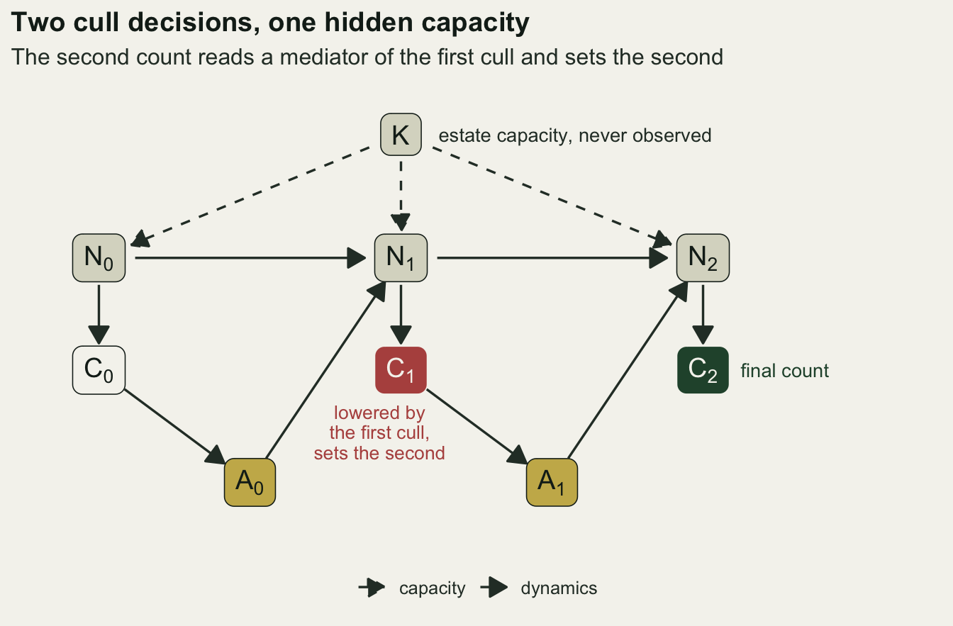

Figure 1: Two cull decisions on one estate. The hidden capacity K drives every true abundance N; each count C reads its N with error; each cull A is set from the count and lowers the next N.

The capacity K adds a second route. It is never observed and it drives every true abundance, and N1 is where it meets the first cull, so conditioning on C1, a descendant of N1, opens the path A0 -> N1 <- K -> N2 -> C2, the kind of path Collider bias and selection opens by conditioning on a common effect. The counting error adds a third twist: C1 is a noisy copy of N1, so holding C1 fixed does not hold N1 fixed, and part of the effect of A0 still leaks through. Those two routes push the all-counts estimate in opposite directions, which a later section measures.

The fix is to model one step at a time. Sequential g-computation, in the iterated conditional expectation form of Bang and Robins (2005), regresses the outcome on the full history up to the last decision, predicts it with the last cull set to the regime, then regresses those predictions on the history up to the decision before, and so on back to the first spring. Each count is conditioned on in the steps for the decisions at and after it, and averaged over, not held fixed, when an earlier cull is set. Inverse probability of treatment weighting (Robins, Hernan and Brumback 2000) breaks the loop from the other side, by reweighting estates so that the culls no longer depend on the counts.

Six estimators on the same record

sum_cull <- function(fit) sum(coef(fit)[c("a0", "a1", "a2")])
top_share <- function(w) if (length(w)) max(w) / sum(w) else NA_real_

ice_mean <- function(rec, set_cull) {
  one <- rep(1, nrow(rec))
  h_2 <- cbind(one, rec$l0, rec$l1, rec$l2, rec$l2^2, rec$a0, rec$a1)
  h_1 <- cbind(one, rec$l0, rec$l1, rec$l1^2, rec$a0)
  h_0 <- cbind(one, rec$l0, rec$l0^2)
  step <- function(h, a_obs, a_set, resp) {
    cf <- .lm.fit(cbind(h, h * a_obs), resp)$coefficients
    drop(cbind(h, h * a_set) %*% cf)
  }
  q_val <- step(h_2, rec$a2, set_cull(rec$l2), rec$y)
  q_val <- step(h_1, rec$a1, set_cull(rec$l1), q_val)
  mean(step(h_0, rec$a0, set_cull(rec$l0), q_val))
}
cull_all     <- function(l) rep(1L, length(l))
cull_none    <- function(l) rep(0L, length(l))
ice_contrast <- function(rec) ice_mean(rec, cull_all) - ice_mean(rec, cull_none)

pop_model <- function(rec) {
  trans <- data.frame(nxt = c(rec$l1, rec$l2, rec$y), now = c(rec$l0, rec$l1, rec$l2),
                      a = c(rec$a0, rec$a1, rec$a2))
  cf <- coef(lm(nxt ~ now + a, trans))
  project <- function(a_set) {
    x_now <- rec$l0
    for (tt in 1:n_dec) x_now <- cf[1] + cf[2] * x_now + cf[3] * a_set
    mean(x_now)
  }
  c(pop = unname(project(1) - project(0)), b_pop = unname(cf[2]), c_pop = unname(cf[3]))
}

estimate_all <- function(rec) {
  long   <- data.frame(a = c(rec$a0, rec$a1, rec$a2), l = c(rec$l0, rec$l1, rec$l2))
  p_den  <- fitted(glm(a ~ l, binomial, long))
  p_num  <- mean(long$a)
  w_step <- ifelse(long$a == 1, p_num / p_den, (1 - p_num) / (1 - p_den))
  w_est  <- apply(matrix(w_step, ncol = n_dec), 1, prod)
  sat    <- lm(y ~ a0 * a1 * a2, rec, weights = w_est)
  ends   <- predict(sat, data.frame(a0 = c(1, 0), a1 = c(1, 0), a2 = c(1, 0)))
  n_cull <- rec$a0 + rec$a1 + rec$a2
  c(unadj    = sum_cull(lm(y ~ a0 + a1 + a2, rec)),
    base     = sum_cull(lm(y ~ a0 + a1 + a2 + l0, rec)),
    allc     = sum_cull(lm(y ~ a0 + a1 + a2 + l0 + l1 + l2, rec)),
    ice      = ice_contrast(rec),
    iptw     = sum_cull(lm(y ~ a0 + a1 + a2, rec, weights = w_est)),
    pop_model(rec),
    iptw_sat = unname(ends[1] - ends[2]),
    w_share  = max(w_est) / sum(w_est),
    w_always = top_share(w_est[n_cull == n_dec]),
    w_never  = top_share(w_est[n_cull == 0]))
}

The first three estimators are what a management record invites. The unadjusted regression puts the three cull indicators on the right and nothing else, and reads the always-minus-never contrast as the sum of the three coefficients. The baseline-adjusted version adds the first count, the analysis of covariance of the baseline-selection post. The all-counts version adds every count before the final one.

The other three model the process. ice_mean() is sequential g-computation: the outcome is regressed on the history with the last cull interacted with everything before it and a squared term in the current count, the fitted model predicts the outcome with the last cull set to the regime, and the predictions become the response for the step before. The working models are ordinary least squares, written with .lm.fit() so that the bootstrap later is fast. The weighted estimator fits one pooled logistic regression of the cull on the current count, which is the form of the true rule, builds stabilised weights as the product over the three years of the marginal cull probability over the fitted one, and fits the additive marginal structural model by weighted least squares; a saturated version with all interactions of the three culls sits beside it as a check on the additive form. The last is the model a population ecologist writes down first: a Gompertz regression of next year’s log count on this year’s and the cull, pooled over estates and years, then projected three years forward from each estate’s first count under always and under never.

The linear case has a formula

Before the Ricker estates, a case where the all-counts answer can be written down. Take the log abundance relative to capacity, x, observed without error, with Gompertz dynamics and the cull before growth:

\[x_{t+1} = b\,(x_t + \delta A_t) + \varepsilon_t, \qquad \delta = \log(1 - h).\]

Unrolling three years gives \(x_3 = b^3 x_0 + \delta\,(b^3 A_0 + b^2 A_1 + b A_2) + \text{noise}\), so always minus never is \(\delta\, b\,(1 + b + b^2)\). The regression on every count sees \(x_3 = b\,x_2 + b\,\delta A_2 + \varepsilon_2\) exactly: once \(x_2\) is held fixed, neither earlier cull nor earlier count carries anything more, and the three cull coefficients sum to \(\delta\, b\). The all-counts estimator therefore recovers the share \(1 / (1 + b + b^2)\) of the effect, the last cull’s direct step and nothing of what the earlier culls did through the counts. At \(b = 0.5\) that is four sevenths.

n_lin <- 200000
b_lin <- 0.5
delta <- log(1 - h_cull)
sim_linear <- function(regime = NULL) {
  x_now <- rnorm(n_lin, 0, sd_init)
  cnt   <- matrix(NA_real_, n_lin, n_dec + 1)
  cull  <- matrix(NA_integer_, n_lin, n_dec)
  for (tt in 1:n_dec) {
    cnt[, tt]  <- x_now
    cull[, tt] <- if (is.null(regime)) {
      rbinom(n_lin, 1, plogis(-0.3 + 1.5 * x_now))
    } else rep(regime, n_lin)
    x_now <- b_lin * (x_now + delta * cull[, tt]) + rnorm(n_lin, 0, sd_proc)
  }
  cnt[, n_dec + 1] <- x_now
  list(cnt = cnt, cull = cull)
}
set.seed(2901)
lin_truth <- mean(sim_linear(1)$cnt[, 4]) - mean(sim_linear(0)$cnt[, 4])
lin_est   <- estimate_all(as_record(sim_linear()))
lin_form_truth <- delta * b_lin * (1 + b_lin + b_lin^2)
lin_form_ratio <- 1 / (1 + b_lin + b_lin^2)
lin_ratio <- lin_est[c("unadj", "base", "allc", "ice", "iptw", "pop")] / lin_truth
round(c(truth = lin_truth, formula = lin_form_truth), 4)

  truth formula 
-0.4484 -0.4470 

round(c(lin_ratio, formula_allc = lin_form_ratio), 3)

       unadj         base         allc          ice         iptw          pop 
       0.743        0.803        0.569        0.996        1.001        0.991 
formula_allc 
       0.571 

With 200000 simulated estates the truth is -0.4484 against the formula’s -0.4470, and the all-counts share is 0.569 against 0.571. The population model is exactly the data-generating model here, and it returns 0.991 of the effect; sequential g-computation returns 0.996. Here the transition the population model fits is the true model of the state, so the population model is a correctly specified g-formula; that is what the Ricker estates take away. The all-counts share is algebra, and the table below prints the formula at the effective slope beside every all-counts row rather than treating the shortfall as something the simulation found.

How different the estates are

The Ricker estates break the linear algebra in three ways at once: the dynamics are curved, the counts carry Poisson error, and the estates differ in capacity by an amount the record does not show. The sweep below holds the rule and the dynamics fixed and moves the spread of log capacity, sd_k, from almost nothing to 0.8, which puts the middle 95 per cent of estates between 1/4.8 and 4.8 times the typical capacity at the top of the sweep. Each cell is 20 simulated management records of 1500 estates, plus side cells with a steeper rule, fewer estates and exact counts. The design constants were fixed before the first run.

n_draw <- 20
cells <- data.frame(
  id      = 1:10,
  sd_k    = c(0.01, 0.2, 0.4, 0.8, 0.4, 0.4, 0.4, 0.01, 0.4, 0.8),
  slope   = c(1.5, 1.5, 1.5, 1.5, 3, 1.5, 1.5, 1.5, 1.5, 1.5),
  n_est   = c(1500, 1500, 1500, 1500, 1500, 500, 150, 1500, 1500, 1500),
  poisson = c(rep(TRUE, 7), rep(FALSE, 3)))

run_cell <- function(i) {
  cl <- cells[i, ]
  out <- lapply(1:n_draw, function(k) {
    seed  <- 1000 * cl$id + 2 * k
    truth <- regime_effect(seed, cl$sd_k, cl$poisson)
    set.seed(seed + 1)
    rec <- as_record(sim_estates(cl$n_est, cl$sd_k, rule_logit(cl$slope), cl$poisson))
    data.frame(id = cl$id, draw = k, truth = truth, t(estimate_all(rec)))
  })
  do.call(rbind, out)
}
sweep_res <- do.call(rbind, lapply(cells$id, run_cell))

est_names <- c("unadj", "base", "allc", "ice", "iptw", "pop", "iptw_sat")
ratio_long <- do.call(rbind, lapply(est_names, function(e)
  data.frame(id = sweep_res$id, draw = sweep_res$draw, estimator = e,
             ratio = sweep_res[[e]] / sweep_res$truth)))
ratio_long <- merge(ratio_long, cells, by = "id")
summ_agg <- aggregate(ratio ~ id + estimator, ratio_long, function(z)
  c(med = median(z), lo = min(z), hi = max(z), mean = mean(z), se = sd(z) / sqrt(length(z))))
summ <- cbind(summ_agg[, 1:2], as.data.frame(summ_agg$ratio))

b_eff_of <- function(tr) uniroot(function(b) delta * b * (1 + b + b^2) - tr, c(0.01, 3))$root
eff <- aggregate(truth ~ id, sweep_res, median)
eff$b_eff   <- sapply(eff$truth, b_eff_of)
eff$formula <- 1 / (1 + eff$b_eff + eff$b_eff^2)
side <- aggregate(cbind(w_share, b_pop, c_pop) ~ id, sweep_res, median)
w_max <- aggregate(w_share ~ id, sweep_res, max)

pick <- function(i, e, what = "med") summ[summ$id == i & summ$estimator == e, what]
mr   <- function(i, e) sprintf("%.2f (%.2f to %.2f)", pick(i, e), pick(i, e, "lo"), pick(i, e, "hi"))

tab_ids <- 1:7
setting <- c("sd_k 0.01", "sd_k 0.2", "sd_k 0.4", "sd_k 0.8", "sd_k 0.4, slope 3",
             "sd_k 0.4, 500 estates", "sd_k 0.4, 150 estates")
med_tab <- data.frame(
  setting     = setting,
  unadjusted  = sapply(tab_ids, pick, e = "unadj"),
  baseline    = sapply(tab_ids, pick, e = "base"),
  all_counts  = sapply(tab_ids, pick, e = "allc"),
  formula     = eff$formula[tab_ids],
  g_comp_ICE  = sapply(tab_ids, pick, e = "ice"),
  IPTW        = sapply(tab_ids, pick, e = "iptw"),
  pop_model   = sapply(tab_ids, pick, e = "pop"),
  max_weight  = side$w_share[tab_ids])
knitr::kable(med_tab, digits = c(0, 2, 2, 2, 2, 2, 2, 2, 3),
             caption = "Median ratio of each estimate to the truth over 20 simulated records (Poisson counts, 1500 estates unless stated). The formula column is 1 / (1 + b + b^2) at the effective slope; max_weight is the median share of the total weight carried by the largest single IPTW weight.")

Median ratio of each estimate to the truth over 20 simulated records (Poisson counts, 1500 estates unless stated). The formula column is 1 / (1 + b + b^2) at the effective slope; max_weight is the median share of the total weight carried by the largest single IPTW weight.

setting	unadjusted	baseline	all_counts	formula	g_comp_ICE	IPTW	pop_model	max_weight
sd_k 0.01	0.70	0.78	0.56	0.48	1.03	0.98	0.84	0.005
sd_k 0.2	0.45	0.69	0.48	0.48	1.00	0.94	0.92	0.006
sd_k 0.4	-0.09	0.62	0.43	0.48	0.98	0.89	1.07	0.009
sd_k 0.8	-1.43	0.60	0.43	0.48	1.02	0.73	1.26	0.021
sd_k 0.4, slope 3	-0.48	0.40	0.44	0.48	1.01	0.83	1.06	0.046
sd_k 0.4, 500 estates	-0.07	0.64	0.47	0.48	1.04	0.87	1.09	0.016
sd_k 0.4, 150 estates	-0.01	0.67	0.47	0.48	1.07	0.86	1.11	0.043

main <- subset(ratio_long, id %in% 1:4)
main_s <- subset(summ, id %in% 1:4)
main_s$sd_k <- cells$sd_k[main_s$id]
lab_map <- c(unadj = "unadjusted", base = "baseline count", allc = "all counts",
             ice = "g-computation (ICE)", iptw = "IPTW", pop = "population model")
off <- c(unadj = -0.025, base = 0, allc = 0.025, ice = -0.025, iptw = 0, pop = 0.025)
main_s <- subset(main_s, estimator %in% names(lab_map))
main_s$x   <- main_s$sd_k + off[main_s$estimator]
main_s$lab <- factor(lab_map[main_s$estimator], levels = lab_map)
est_col <- c("unadjusted" = te_rust, "baseline count" = te_gold, "all counts" = te_forest,
             "g-computation (ICE)" = te_forest, "IPTW" = te_gold, "population model" = te_rust)
est_shape <- c("unadjusted" = 17, "baseline count" = 15, "all counts" = 16,
               "g-computation (ICE)" = 16, "IPTW" = 15, "population model" = 17)
form_line <- mean(eff$formula[1:4])

panel_sweep <- function(keys, title, form = FALSE) {
  d <- subset(main_s, estimator %in% keys)
  p <- ggplot(d, aes(x = x, y = med, colour = lab, shape = lab)) +
    geom_hline(yintercept = 1, colour = te_ink, linewidth = 0.5) +
    geom_hline(yintercept = 0, colour = te_line, linewidth = 0.5) +
    geom_errorbar(aes(ymin = lo, ymax = hi), width = 0, linewidth = 0.6) +
    geom_line(linewidth = 0.6) +
    geom_point(size = 2.6) +
    scale_colour_manual(values = est_col, name = NULL) +
    scale_shape_manual(values = est_shape, name = NULL) +
    scale_x_continuous(breaks = c(0.01, 0.2, 0.4, 0.8)) +
    labs(x = "sd of log capacity across estates", y = "estimate / truth", title = title) +
    theme_datasheet() +
    theme(legend.position = "bottom", legend.direction = "vertical")
  if (form) p <- p + geom_hline(yintercept = form_line, linetype = "dashed", colour = te_forest) +
    annotate("text", x = 0.62, y = 0.22, label = "dashed: 1 / (1 + b + b^2)\nat the effective slope",
             colour = te_forest, size = 3.3)
  p
}
(panel_sweep(c("unadj", "base", "allc"), "Regressions on the record", form = TRUE) |
   panel_sweep(c("ice", "iptw", "pop"), "Models of the process")) +
  plot_annotation(theme = theme_datasheet())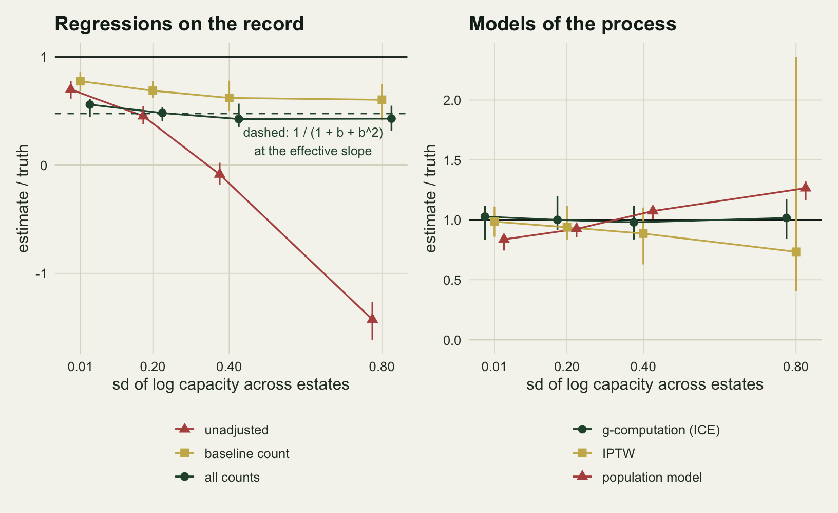

Figure 2: Ratio of each estimate to the true always-minus-never effect against the spread of estate capacity, for 1500 estates with Poisson counts: median and range over 20 simulated records.

The unadjusted regression is the estimator whose answer depends most on the estates. With almost no spread in capacity it reads 0.70 (0.61 to 0.78) of the effect, median and range over the 20 records: culling appears to work, but less than it does, because the estates that culled were the ones that had counted high. At a spread of 0.2 it reads 0.45 (0.38 to 0.54), at 0.4 -0.09 (-0.18 to 0.02), and at 0.8 -1.43 (-1.61 to -1.27): at the top of the sweep the culled estates end with more deer than the unculled ones, by more than the true effect in the other direction. The mechanism is plain. A large estate holds many deer, counts high and culls often, so the regression compares big culled estates with small unculled ones, and the more the estates differ, the more the capacity difference outweighs the cull. The sign of the naive answer is set by how alike the estates are, and a record from any one region shows one point on this curve.

The first count removes part of that, because it is a proxy for capacity: the baseline-adjusted median falls from 0.78 to 0.60 across the sweep instead of changing sign. The all-counts regression reads 0.43 (0.35 to 0.57) in the main setting (spread 0.4, 1500 estates), beside 0.476 from the formula at the effective slope defined in the next section, and its medians stay between 0.43 and 0.56 over the four spreads. That shortfall is mostly the algebra of the previous section.

On the right, sequential g-computation has medians between 0.98 and 1.03 at 1500 estates, with Monte Carlo standard errors of the mean ratio between 0.016 and 0.019. That is Robins’s result doing what it says, not a finding of this post. The two other process estimators are where the measurement lies. The population model drifts from 0.84 (0.74 to 0.87) with no spread to 1.26 (1.16 to 1.32) at 0.8, with standard errors of the mean of at most 0.010, so it crosses the truth somewhere between spreads of 0.2 and 0.4 and is wrong on either side. The weighted estimator falls from 0.98 to 0.73 in median while its range widens to 0.40 to 2.36. The steeper rule (slope 3, spread 0.4) pushes the unadjusted ratio to -0.48 and the weighted one to 0.83 (0.47 to 1.90), and leaves g-computation at 1.01.

Capacity and counting error move the all-counts share

The formula needs a slope, and the Ricker has no single one. On the log scale next year’s abundance changes with this year’s at slope 1 - rN/K, which equals 0.5 only at capacity and is closer to one below it, where culled populations spend their time. Solving the simulated truth for b in the linear formula, truth = delta b (1 + b + b^2), gives an effective slope. With exact counts and almost no spread in capacity the truth is -0.719, the effective slope 0.667 and the formula share 0.474. The effective slope is read off the truth, so agreement is a consistency check on the algebra rather than an independent prediction, and it is the only cell where the linear argument should hold. The side cells with exact counts (poisson = FALSE) let the two ingredients the linear case lacks be switched on one at a time.

dec <- subset(ratio_long, id %in% c(1, 3, 4, 8, 9, 10) & estimator %in% c("allc", "pop"))
dec$counts <- ifelse(dec$poisson, "Poisson counts", "exact counts")
dec$panel  <- ifelse(dec$estimator == "allc", "Adjust for every count", "Population model")
dec_med <- aggregate(ratio ~ sd_k + counts + panel, dec, median)
form_exact <- mean(eff$formula[8:10])
ggplot(dec, aes(x = factor(sd_k), y = ratio, colour = counts)) +
  geom_hline(yintercept = 1, colour = te_ink, linewidth = 0.5) +
  geom_hline(data = data.frame(panel = "Adjust for every count", yint = form_exact),
             aes(yintercept = yint), linetype = "dashed", colour = te_forest) +
  geom_point(position = position_jitterdodge(jitter.width = 0.15, dodge.width = 0.6, seed = 3),
             alpha = 0.55, size = 1.6) +
  geom_point(data = dec_med, position = position_dodge(width = 0.6), shape = 95, size = 12) +
  facet_wrap(~ panel, scales = "free_y") +
  scale_colour_manual(values = c("exact counts" = te_forest, "Poisson counts" = te_rust), name = NULL) +
  labs(x = "sd of log capacity across estates", y = "estimate / truth",
       title = "Capacity spread and counting error pull in different directions") +
  theme_datasheet() +
  theme(legend.position = "bottom",
        strip.text = element_text(colour = te_ink, face = "bold"))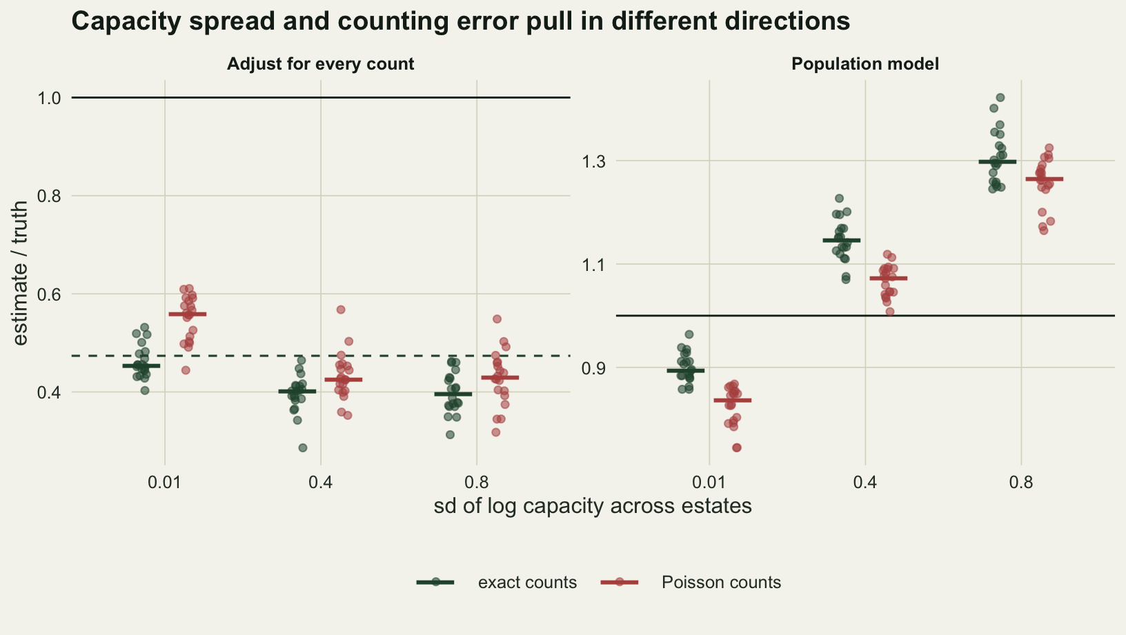

Figure 3: All-counts and population-model estimates as a ratio to the truth, with exact and with Poisson counts, at three spreads of estate capacity (20 simulated records of 1500 estates per point cloud).

With exact counts and no spread, the all-counts median is 0.45 (0.40 to 0.53) against the formula’s 0.474. The mean ratio, 0.462, sits 1.6 Monte Carlo standard errors below the formula, so in this cell the linear argument accounts for the shortfall to within what 20 records can resolve. Spreading capacity lowers the median, to 0.40 at 0.4 and 0.40 at 0.8 with exact counts, against a formula value of 0.474 at both; the fall happens by 0.4, and the medians at 0.4 and 0.8 differ by less than the Monte Carlo standard error of either mean ratio (0.009 and 0.009). The hidden capacity drives every count, so holding a count fixed opens the path from an earlier cull into the abundance that count reads, back to K and on to the final count, and the estimate is pulled away from the truth. Poisson counting raises it again, to 0.56, 0.43 and 0.43 at the three spreads: a count with error is an incomplete stand-in for the abundance, so conditioning on it blocks only part of the mediated path and lets some of the earlier culls’ effect back in. The rise is largest when the estates are alike, where the same counting error is a larger share of the variation between counts. Which force wins depends on the spread and on the counting precision, so the all-counts share of a real record cannot be read off the formula.

The right panel belongs to the next section, but the same switch works there. Counting error pulls the population model down at every spread, from 0.89 to 0.84 with no spread and from 1.30 to 1.26 at 0.8.

The population model is a g-formula with one slope

The population model is a g-formula. It models each year’s count given the last year’s count and the cull, then iterates that model forward under each regime, which is exactly what Robins’s formula prescribes, with a Markov assumption on the state and one straight line for every estate. Because the projection is linear, its answer is an identity in the two fitted coefficients: with a pooled slope b and a cull coefficient c, always minus never is c (1 + b + b^2), whatever the data.

id_gap <- max(abs(sweep_res$pop - sweep_res$c_pop * (1 + sweep_res$b_pop + sweep_res$b_pop^2)))
pop_tab <- data.frame(sd_k = cells$sd_k[1:4], b_pop = side$b_pop[1:4], c_pop = side$c_pop[1:4],
                      ratio = sapply(1:4, pick, e = "pop"))
knitr::kable(pop_tab, digits = 3,
             caption = "Median pooled slope, cull coefficient and ratio to the truth of the population model, Poisson counts, 1500 estates.")

Median pooled slope, cull coefficient and ratio to the truth of the population model, Poisson counts, 1500 estates.

sd_k	b_pop	c_pop	ratio
0.01	0.552	-0.319	0.837
0.20	0.645	-0.318	0.924
0.40	0.795	-0.315	1.074
0.80	0.928	-0.320	1.265

The identity holds in every record up to floating-point rounding, so the drift is all in the two coefficients. The cull coefficient barely moves, staying between -0.320 and -0.315, while the pooled slope climbs from 0.55 to 0.93. A regression pooled over estates without an estate term reads lasting differences in capacity as persistence: an estate that counts high this year counts high next year because its K is high, and the pooled line cannot tell that from a population that returns to its equilibrium slowly. A steeper slope carries the cull’s effect further forward, and the projection overshoots.

With no spread the model falls short instead, and two things account for it. Counting error flattens the pooled slope, the bias the Gompertz state-space model is built to remove: with exact counts the slope is 0.62 and the ratio 0.895, with Poisson counts 0.55 and 0.837. What remains with exact counts is a straight Gompertz line fitted through curved Ricker dynamics, whose slope 0.62 sits below the effective slope 0.67 read off the truth. So the population model is right when the estates are alike, the counts are precise and the dynamics are close to its line, and the error it makes otherwise has a direction set by the estates.

Weights that need both histories

w_hist  <- aggregate(cbind(w_always, w_never) ~ id, sweep_res, median)
wide8   <- subset(sweep_res, id == 4)
miss8   <- abs(wide8$iptw / wide8$truth - 1)
n_miss8 <- sum(miss8 > 0.2)
n_quiet <- sum(miss8 > 0.2 & wide8$w_share <= 0.03)
rho8    <- sapply(c("w_share", "w_always", "w_never"), function(v)
  cor(wide8[[v]], miss8, method = "spearman"))
round(c(missed = n_miss8, missed_quiet = n_quiet, rho8), 2)

      missed missed_quiet      w_share     w_always      w_never 
       14.00        12.00        -0.04        -0.14         0.25 

The weighted estimator asks each estate to stand in for the estates like it that took the other decisions. With stabilised weights the largest single weight carries a median 0.005 of the total with no spread in capacity and 0.021 at 0.8; in the worst record at 0.8 it carries 0.137, and with the steeper rule 0.221. The rule never sets a probability of exactly zero or one, so positivity holds in principle, and with the treatment model of the right form the weighting is consistent. In practice an estate with a high capacity counts high every spring and culls almost every year, so a never-culled history on a large estate is rare, and so is an always-culled history on a small one, which counts low and seldom culls. The few estates with those histories carry the weight of all the others, the always-culled ones most heavily here. Measured within its own history rather than against the whole record, the largest weight carries a median 0.106 of the always-culled weight at a spread of 0.4 and 0.166 at 0.8, against 0.032 and 0.082 of the never-culled weight. The median ratio already sits below the truth at a spread of 0.4 (mean 0.897, Monte Carlo standard error 0.026) and falls to 0.73 at 0.8, with 1500 estates in the record.

The additive structural model is not the cause. The saturated version, with a separate mean for every one of the eight cull histories, reads 0.83 at 0.4 and 0.58 at 0.8, no better; it leans harder on the two extreme histories, which are the ones the weights struggle to fill. The propensity-score post’s overlap section makes the same point for one treatment. With three treatments the propensities multiply, and near-violations compound across years.

A record of a hundred and fifty estates

A real management record might cover a hundred or so estates, not 1500. With 150 estates at a spread of 0.4, g-computation reads 1.07 (0.51 to 1.49), the weighted estimator 0.86 (0.51 to 1.28), the population model 1.11 (0.94 to 1.33) and the all-counts regression 0.47 (0.27 to 0.77). The estimate is still centred near the truth for g-computation, but any single record can be half or one and a half times it, so the honest answer from 150 estates is the direction and a rough size, with a wide interval.

The interval comes from a bootstrap over estates: resample the estates with replacement, rerun the whole sequence of regressions, take percentiles. The chunk below does it once on a record of 500 estates and then checks the coverage of the percentile interval over 50 such records.

boot_ice <- function(rec, n_boot = 200) {
  vapply(1:n_boot, function(b) ice_contrast(rec[sample.int(nrow(rec), replace = TRUE), ]), 0)
}
set.seed(6101)
rec_500   <- as_record(sim_estates(500, 0.4, rule_logit(1.5)))
bs_500    <- boot_ice(rec_500)
truth_500 <- regime_effect(6100, 0.4)
est_500   <- ice_contrast(rec_500)
ci_500    <- quantile(bs_500, c(0.025, 0.975))

cover <- t(sapply(1:50, function(k) {
  seed <- 7000 + 2 * k
  tr   <- regime_effect(seed, 0.4)
  set.seed(seed + 1)
  rec  <- as_record(sim_estates(500, 0.4, rule_logit(1.5)))
  ci   <- quantile(boot_ice(rec), c(0.025, 0.975))
  c(truth = tr, lo = ci[[1]], hi = ci[[2]])
}))
cov_rate  <- mean(cover[, "lo"] <= cover[, "truth"] & cover[, "truth"] <= cover[, "hi"])
cov_se    <- sqrt(cov_rate * (1 - cov_rate) / nrow(cover))
width_rel <- median((cover[, "hi"] - cover[, "lo"]) / abs(cover[, "truth"]))

nd <- subset(ratio_long, id %in% c(3, 6, 7) & estimator %in% c("ice", "iptw", "pop"))
nd$lab <- factor(lab_map[nd$estimator], levels = lab_map[c("ice", "iptw", "pop")])
nd_med <- aggregate(ratio ~ n_est + lab, nd, median)
ggplot(nd, aes(x = factor(n_est), y = ratio, colour = lab)) +
  geom_hline(yintercept = 1, colour = te_ink, linewidth = 0.5) +
  geom_point(position = position_jitter(width = 0.12, height = 0, seed = 4), alpha = 0.6, size = 1.7) +
  geom_point(data = nd_med, shape = 95, size = 13, colour = te_ink) +
  facet_wrap(~ lab) +
  scale_colour_manual(values = est_col, guide = "none") +
  labs(x = "estates in the management record", y = "estimate / truth",
       title = "Fewer estates, wider scatter") +
  theme_datasheet() +
  theme(strip.text = element_text(colour = te_ink, face = "bold"))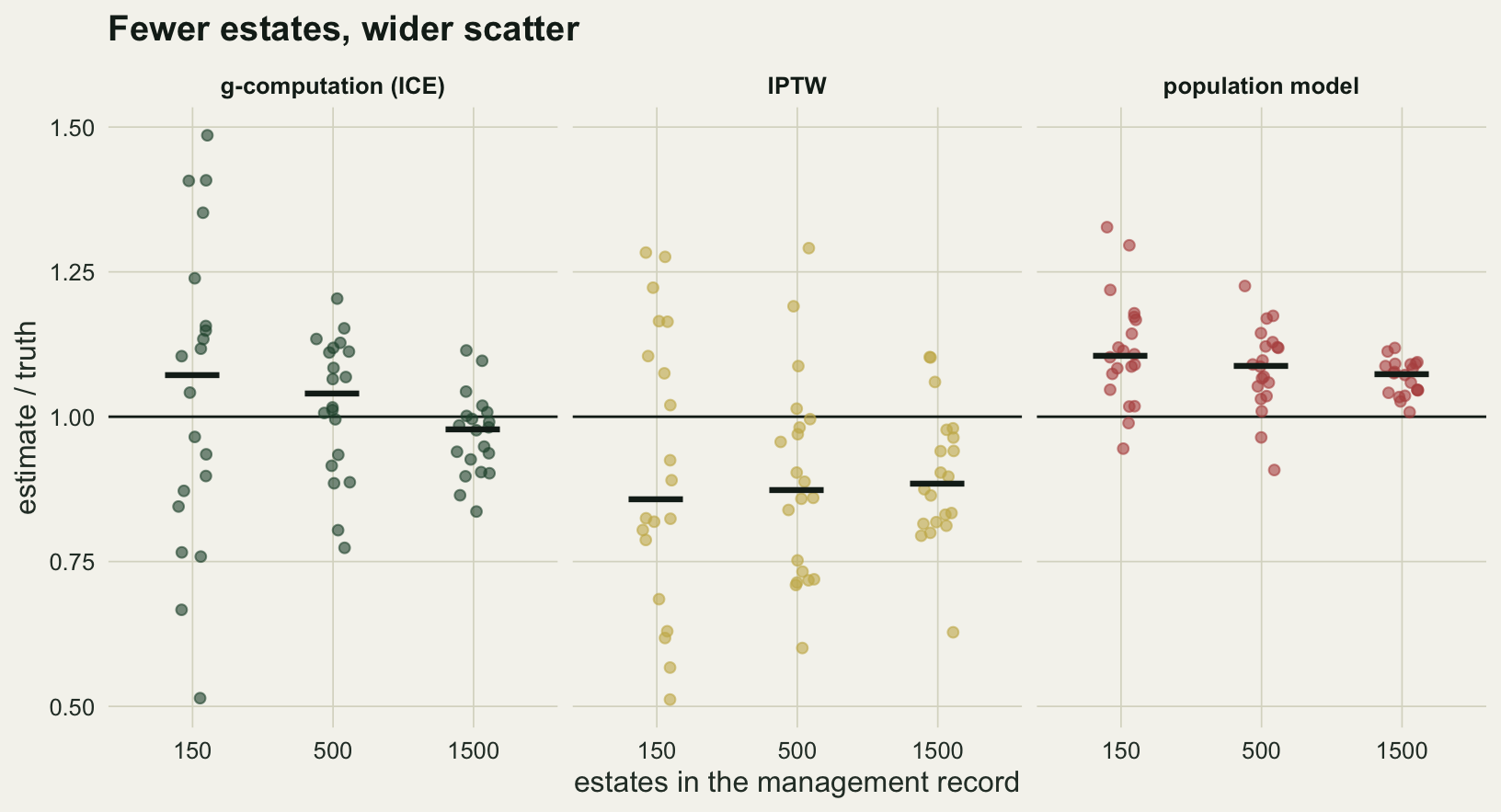

Figure 4: Ratio to the truth of the three process-based estimators in each of 20 simulated records, for 150, 500 and 1500 estates at a log-capacity spread of 0.4; bars mark the medians.

On the single record the estimate is -0.658 against a truth of -0.711, and the 95 per cent percentile interval runs from -0.828 to -0.512. Over 50 records the interval covered the truth in a share 0.94 of them (Monte Carlo standard error 0.034), with a median width of 0.44 times the size of the effect. At 500 estates, then, the bootstrap interval is honest and wide.

The figure shows the trade between the process estimators. The population model scatters least at every size, but its centre stays above the truth, from 1.11 at 150 estates to 1.07 at 1500. The weighted estimator’s median stays below one at every size, from 0.86 to 0.89. G-computation scatters most at 150 estates and tightens as the record grows.

A threshold rule instead of always and never

Always against never is the textbook contrast, and not what a deer management group would vote on. The policy on the table is more likely a rule: cull whenever the spring count is above 80. Sequential g-computation handles a rule of that kind without new machinery, because each step sets the cull from the rule applied to the count at that step, which is why ice_mean() takes a function of the count rather than a fixed value. The truth comes from running the rule itself in the simulator. The last block in the chunk asks a different question: what if the record itself came from a rule with no randomness in it, every estate culling exactly when its count was above 80?

thr_count  <- 80
cull_above <- function(l) as.integer(l > log(thr_count + 1))
sd_set     <- c(0.01, 0.4, 0.8)
dyn <- do.call(rbind, lapply(seq_along(sd_set), function(j) do.call(rbind, lapply(1:20, function(k) {
  seed <- 8000 + 100 * j + 2 * k
  tr   <- regime_effect(seed, sd_set[j], arm1 = function(l, u) cull_above(l))
  set.seed(seed + 1)
  rec  <- as_record(sim_estates(1500, sd_set[j], rule_logit(1.5)))
  est  <- ice_mean(rec, cull_above) - ice_mean(rec, cull_none)
  data.frame(sd_k = sd_set[j], truth = tr, ratio = est / tr, diff = est - tr)
}))))
dyn_med <- aggregate(cbind(truth, ratio, diff) ~ sd_k, dyn, median)
dyn_rng <- aggregate(ratio ~ sd_k, dyn, range)

dyn_big <- sapply(1:3, function(k) {
  tr  <- regime_effect(8900 + 2 * k, 0.4, arm1 = function(l, u) cull_above(l))
  set.seed(8901 + 2 * k)
  rec <- as_record(sim_estates(n_big, 0.4, rule_logit(1.5)))
  (ice_mean(rec, cull_above) - ice_mean(rec, cull_none)) / tr
})

det_res <- do.call(rbind, lapply(seq_along(sd_set), function(j) do.call(rbind, lapply(1:20, function(k) {
  seed <- 9000 + 100 * j + 2 * k
  tr   <- regime_effect(seed, sd_set[j])
  set.seed(seed + 1)
  rec  <- as_record(sim_estates(1500, sd_set[j], function(l, u) cull_above(l)))
  data.frame(sd_k = sd_set[j], ice = ice_contrast(rec) / tr, pop = pop_model(rec)[["pop"]] / tr)
}))))
det_med <- aggregate(cbind(ice, pop) ~ sd_k, det_res, median)
det_lo  <- aggregate(cbind(ice, pop) ~ sd_k, det_res, min)
det_hi  <- aggregate(cbind(ice, pop) ~ sd_k, det_res, max)

The rule culls only the estates that count high, so its effect is smaller than always culling: a median truth of -0.152, -0.191 and -0.245 at spreads of 0.01, 0.4 and 0.8. G-computation overshoots it, with median ratios 1.10, 1.11 and 1.13 and ranges from 0.85 to 1.33; on the log scale the median error is between -0.015 and -0.031. Three records of 20000 estates at 0.4 give 1.08, 1.07 and 1.07, so the overshoot is not small-sample noise. A plausible source is the working models: the rule puts a jump into the predicted outcome at the threshold, and a quadratic in the count cannot follow it. Richer working models were not tried here.

When the record comes from the deterministic rule, positivity fails outright. No estate above the threshold was left alone and none below it was culled, every propensity is zero or one, and the weighted estimator cannot be computed. G-computation still returns a number, by extrapolating each working model across the threshold into histories the record never contains, and the number is unreliable: median ratios of 1.17, 1.01 and 1.05 at the three spreads, with single records ranging from -0.31 to 2.55 when the estates are alike. The population model is steadier under the same record, 0.77, 1.02 and 1.19, because its single straight line extrapolates smoothly; it carries the same capacity drift as before. A record in which the managers never departed from their rule cannot say what departing from it would have done, except through a model’s shape.

What to report

Say how each cull decision was made and what it read. If it read the count, the regression of the final count on the cull history, with or without the counts, does not estimate the effect of culling, and a paper that reports it should say which of the two failures it has: the unadjusted version is confounded by whatever makes estates differ, and the version adjusted for every count keeps only the last step, a share 1 / (1 + b + b^2) of the effect in the linear case.

Name the regime the estimate refers to. Always against never is the simplest contrast; a threshold rule is a different estimand with a smaller effect, and g-computation estimates either with the same code.

Report sequential g-computation with its working models written out (which history terms, which interactions), and a bootstrap interval over estates, not over estate-years. At 500 estates the percentile interval covered the truth at close to its nominal rate here.

If a population model is used instead, say whether the estates differ in capacity and whether the counts carry error, report the pooled slope beside the cull coefficient, and remember that the projected effect is c (1 + b + b^2): an inflated slope inflates the effect.

If weights are used, report the largest weight as a share of the weight within each extreme history (always culled, never culled), not only of the whole record, where it is diluted: at a spread of 0.8 the whole-record share stayed at or below 0.03 in 12 of the 14 records whose weighted estimate missed the truth by more than a fifth. Neither share is a pass mark. Over all 20 records at that spread the rank correlation between the size of the miss and the largest weight’s share was -0.04 for the whole record, -0.14 within the always-culled history and 0.25 within the never-culled one. Put the weighted estimate beside g-computation and beside a saturated structural model, and read a gap between them as the warning.

Honest limits

The record has three decisions and one outcome. With T decisions the linear algebra gives the all-counts share 1 / (1 + b + … + b^(T - 1)), so longer records lose more, but the capacity drift of the population model and the weight problem of IPTW over longer records were not measured.

The cull rule reads the count and nothing else. A real stalker also reads the damage to woodland, complaints from neighbours and last year’s cull; anything of that kind which also drives the deer and is missing from the record is an unmeasured confounder, and sequential g-computation needs sequential exchangeability as much as any other method does.

Capacity is fixed within an estate and the estates do not exchange deer. Neighbouring estates share animals in reality, so one estate’s cull changes its neighbour’s count, which is interference between units and outside everything shown here.

The working models of g-computation are quadratics in the count with the current cull interacted with the history. They were close enough for always against never and not for the threshold rule, where an overshoot of 0.07 to 0.08 of the effect persisted with 20000 estates. Nothing here shows how to choose them; a flexible learner in each step, or the estimators that combine the outcome models with the weights, which grew from Bang and Robins (2005), would be the next thing to try.

The population model was fitted in its simplest pooled form. An estate intercept would absorb the capacity differences in principle, but with four counts per estate a fixed-effect autoregression has a known short-panel bias of its own, and neither that nor a random-intercept version was run. The state-space repair for counting error was not combined with it either.

All effects are on the scale of mean log(count + 1), which is what a Gompertz analysis would use. The same record analysed on the count scale would give different ratios, and the Poisson error on log(count + 1) is not the error model of a real deer count, which carries detection and double counting.

Bootstrap coverage was measured in one setting, 500 estates at a spread of 0.4, over 50 records; its Monte Carlo standard error is 0.034, which is too coarse to tell 0.90 from 0.95.

References

Robins JM 1986 Mathematical Modelling 7(9-12):1393-1512 (10.1016/0270-0255(86)90088-6)

Robins JM, Hernan MA, Brumback B 2000 Epidemiology 11(5):550-560 (10.1097/00001648-200009000-00011)

Bang H, Robins JM 2005 Biometrics 61(4):962-973 (10.1111/j.1541-0420.2005.00377.x)

Daniel RM, Cousens SN, De Stavola BL, Kenward MG, Sterne JAC 2013 Statistics in Medicine 32(9):1584-1618 (10.1002/sim.5686)

Larsen AE, Meng K, Kendall BE 2019 Methods in Ecology and Evolution 10(7):924-934 (10.1111/2041-210X.13190)

Related tutorials

• G-computation and standardisation
• Confounding and backdoor adjustment
• Propensity scores and IPW
• Detecting density dependence in R