G-computation and standardisation

Standardisation and the g-formula for a marginal causal effect in R: fit an outcome model, predict potential outcomes under each treatment level, then average.

Suppose you have observational data on a management action and an ecological outcome, and you have measured the variables that drive both. Adjusting for those confounders in a regression is the usual move, and the earlier tutorial on inverse-probability weighting did it by modelling the treatment. This tutorial takes the other route: model the outcome, then use the fitted model to predict what would have happened to every unit under each treatment level, and average. That procedure is standardisation, also called the g-formula. It returns a marginal (population-average) effect, and it exposes a subtlety that a regression coefficient hides: for a nonlinear model the coefficient is not the population effect.

A confounded example

Three covariates drive both a binary treatment d and a binary outcome y. The treatment has a true conditional log-odds effect bD, so the true conditional odds ratio is exp(bD). Because the covariates push units towards treatment and towards the outcome at the same time, the raw association is confounded.

b0 <- -0.5; bD <- log(2.5); b1 <- 1.0; b2 <- 0.8; b3 <- 0.7   # outcome model
a0 <- -0.4; a1 <- 0.8; a2 <- 0.5; a3 <- 0.6                    # treatment model (confounding)

gen <- function(n) {
  x1 <- rnorm(n); x2 <- rnorm(n); x3 <- rbinom(n, 1, 0.5)
  d  <- rbinom(n, 1, expit(a0 + a1*x1 + a2*x2 + a3*x3))
  y  <- rbinom(n, 1, expit(b0 + bD*d + b1*x1 + b2*x2 + b3*x3))
  data.frame(y, d, x1, x2, x3)
}

# true SAMPLE-marginal effect (uses the known coefficients on this covariate set)
true_marg <- function(dat) {
  p1 <- expit(b0 + bD*1 + b1*dat$x1 + b2*dat$x2 + b3*dat$x3)
  p0 <- expit(b0 + bD*0 + b1*dat$x1 + b2*dat$x2 + b3*dat$x3)
  m1 <- mean(p1); m0 <- mean(p0)
  c(RD = m1 - m0, RR = m1 / m0, OR = (m1/(1-m1)) / (m0/(1-m0)))
}

set.seed(166)
n <- 2000
dat <- gen(n)
c(prev_D = mean(dat$d), prev_Y = mean(dat$y))
#> prev_D prev_Y 
#> 0.4985 0.5505

The true conditional odds ratio is 2.5. Averaging the known potential-outcome probabilities over this sample gives the marginal targets the analysis should recover.

tm <- true_marg(dat)
round(tm, 4)                # marginal risk difference, risk ratio, odds ratio
#>     RD     RR     OR 
#> 0.1651 1.3456 1.9677

So on this sample the true marginal risk difference is 0.165 and the true marginal odds ratio is 1.968, which is already pulled towards one relative to the conditional odds ratio of 2.5. Hold that thought.

Naive and adjusted regression

The unadjusted odds ratio is badly confounded. Adjusting for the covariates fixes the confounding and recovers the conditional effect.

m_naive <- glm(y ~ d, family = binomial, data = dat)
OR_naive <- exp(coef(m_naive)["d"])
ci_naive <- exp(coef(m_naive)["d"] + c(-1, 1) * 1.96 * summary(m_naive)$coef["d", "Std. Error"])

m_adj <- glm(y ~ d + x1 + x2 + x3, family = binomial, data = dat)
OR_cond <- exp(coef(m_adj)["d"])
ci_cond <- exp(coef(m_adj)["d"] + c(-1, 1) * 1.96 * summary(m_adj)$coef["d", "Std. Error"])

c(OR_naive = OR_naive, OR_conditional = OR_cond)
#>       OR_naive.d OR_conditional.d 
#>         5.023772         2.900115

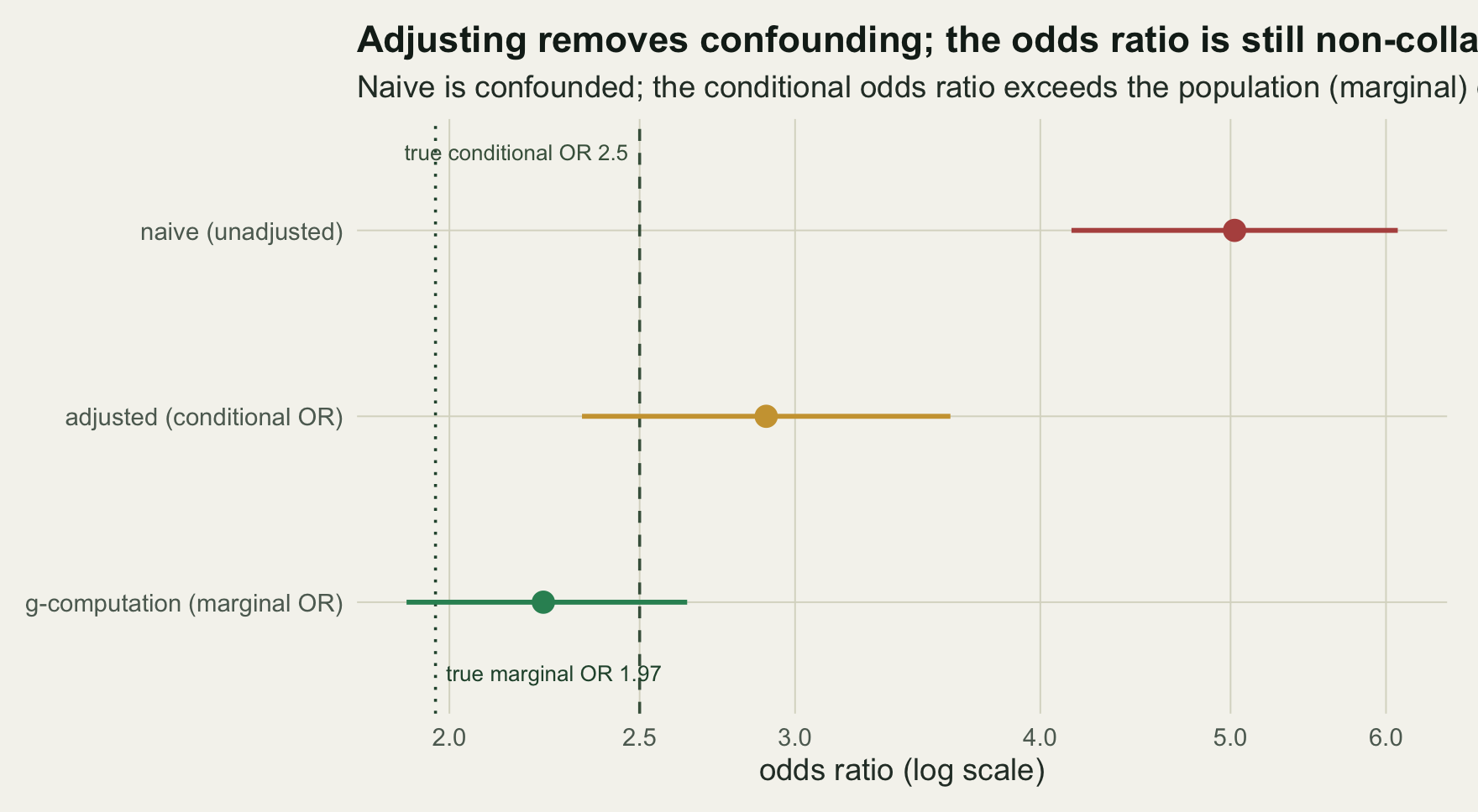
The naive odds ratio is 5.02 (95% CI 4.15 to 6.08), far above the truth: high-covariate units both receive the treatment and have the outcome, and the unadjusted comparison charges that to the treatment. The adjusted odds ratio is 2.90 (95% CI 2.34 to 3.60), which covers the true conditional value of 2.5. The confounding is handled.

The conditional coefficient is not the population effect

Here is the catch. The adjusted coefficient is the odds ratio holding the covariates fixed: it compares two units with the same covariates. The odds ratio is not collapsible, meaning the covariate-adjusted (conditional) odds ratio and the population-averaged (marginal) odds ratio differ even when there is no confounding at all (Greenland, Robins and Pearl 1999). With a prognostic covariate the conditional odds ratio sits further from one than the marginal odds ratio. So if the question is population-level (“how much would the outcome frequency change if everyone were treated?”), the adjusted coefficient answers a different question.

Standardisation answers the population question directly. Fit the outcome model, then for every unit predict the outcome probability twice, once setting d = 1 and once setting d = 0, and average each set. The contrast of the two averages is the marginal effect on whatever scale you choose.

gcomp <- function(model, dat) {
  d1 <- transform(dat, d = 1); d0 <- transform(dat, d = 0)
  mu1 <- predict(model, d1, type = "response")
  mu0 <- predict(model, d0, type = "response")
  m1 <- mean(mu1); m0 <- mean(mu0)
  list(RD = m1 - m0, RR = m1 / m0, OR = (m1/(1-m1)) / (m0/(1-m0)),
       mu1 = mu1, mu0 = mu0, d1 = d1, d0 = d0)
}
g <- gcomp(m_adj, dat)
c(RD = g$RD, RR = g$RR, OR = g$OR)
#>        RD        RR        OR 
#> 0.1957107 1.4283812 2.2330064

Standardisation gives a marginal risk difference of 0.196, a marginal risk ratio of 1.428, and a marginal odds ratio of 2.23. Compare the two odds ratios from the same adjusted model: conditional 2.90 against marginal 2.23, a ratio of 1.30. Nothing is wrong; the two numbers simply answer different questions, and only the marginal one is comparable to a risk difference or a risk ratio. The risk difference and the risk ratio are collapsible, so for them the conditional-versus-marginal gap does not arise in the same way; the standardised values are just the population averages.

set.seed(1660)
B <- 1000; bs_or <- numeric(B)
for (b in 1:B) {
  idx <- sample.int(n, n, replace = TRUE); db <- dat[idx, ]
  mb <- glm(y ~ d + x1 + x2 + x3, family = binomial, data = db)
  bs_or[b] <- gcomp(mb, db)$OR
}
ci_OR_boot <- quantile(bs_or, c(.025, .975))

lev <- c("g-computation (marginal OR)", "adjusted (conditional OR)", "naive (unadjusted)")
est_df <- data.frame(
  label = factor(c("naive (unadjusted)", "adjusted (conditional OR)", "g-computation (marginal OR)"), levels = lev),
  or = c(OR_naive, OR_cond, g$OR),
  lo = c(ci_naive[1], ci_cond[1], ci_OR_boot[1]),
  hi = c(ci_naive[2], ci_cond[2], ci_OR_boot[2]),
  kind = c("naive", "conditional", "marginal"))

ggplot(est_df, aes(or, label, colour = kind)) +
  geom_vline(xintercept = exp(bD), linetype = "dashed", colour = te$label) +
  geom_vline(xintercept = tm["OR"], linetype = "dotted", colour = te$forest) +
  geom_pointrange(aes(xmin = lo, xmax = hi), linewidth = 0.9, size = 0.7) +
  annotate("text", x = exp(bD), y = 3.42, label = "true conditional OR 2.5", hjust = 1.05, size = 3, colour = te$label) +
  annotate("text", x = tm["OR"], y = 0.62, label = "true marginal OR 1.97", hjust = -0.05, size = 3, colour = te$forest) +
  scale_colour_manual(values = c(naive = te$abandoned, conditional = te$grazed, marginal = te$mown), guide = "none") +
  scale_x_log10(breaks = c(1.5, 2, 2.5, 3, 4, 5, 6)) +
  labs(x = "odds ratio (log scale)", y = NULL,
       title = "Adjusting removes confounding; the odds ratio is still non-collapsible",
       subtitle = "Naive is confounded; the conditional odds ratio exceeds the population (marginal) odds ratio") +
  theme_te()

Figure 1: Three odds ratio estimates with 95% intervals. The naive estimate is confounded; the adjusted conditional odds ratio recovers the true conditional value but exceeds the population (marginal) odds ratio from standardisation.

Uncertainty

The standardised estimate is a nonlinear function of every coefficient and of the covariate distribution, so its standard error is not any single coefficient standard error. Two routes agree here. The delta method propagates the coefficient covariance through the gradient of the risk difference, treating the covariates as fixed (this targets the sample-standardised estimand). The nonparametric bootstrap resamples rows, so it also carries covariate sampling and targets the population estimand.

gcomp_rd_se <- function(model, g) {
  X1 <- model.matrix(delete.response(terms(model)), g$d1)
  X0 <- model.matrix(delete.response(terms(model)), g$d0)
  grad <- colMeans(g$mu1*(1-g$mu1)*X1) - colMeans(g$mu0*(1-g$mu0)*X0)
  sqrt(as.numeric(t(grad) %*% vcov(model) %*% grad))
}
se_delta <- gcomp_rd_se(m_adj, g)
ci_delta <- g$RD + c(-1, 1) * 1.96 * se_delta

set.seed(1660)                    # same stream as the OR bootstrap above
bs_rd <- numeric(B)
for (b in 1:B) {
  idx <- sample.int(n, n, replace = TRUE); db <- dat[idx, ]
  mb <- glm(y ~ d + x1 + x2 + x3, family = binomial, data = db)
  bs_rd[b] <- gcomp(mb, db)$RD
}
c(delta_SE = se_delta, boot_SE = sd(bs_rd))
#>   delta_SE    boot_SE 
#> 0.02074907 0.02017871
round(rbind(delta = ci_delta, bootstrap = quantile(bs_rd, c(.025, .975))), 4)
#>             2.5%  97.5%
#> delta     0.1550 0.2364
#> bootstrap 0.1574 0.2354

The delta-method standard error is 0.021 and the bootstrap standard error is 0.020; the intervals nearly coincide, with the bootstrap a touch wider because it also accounts for resampling the covariates. Either way the marginal risk difference is estimated at 0.196, close to the true 0.165.

It is unbiased across datasets

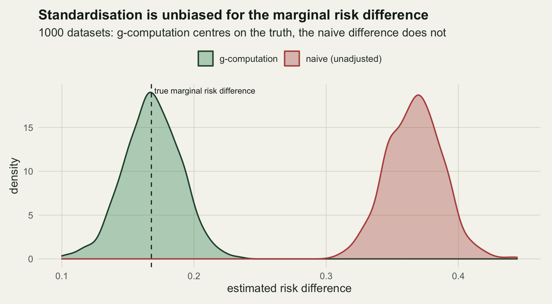
One sample can be lucky. Repeating the whole procedure over many simulated datasets shows that standardisation is unbiased for the marginal risk difference with close to nominal interval coverage, while the naive unadjusted difference is badly biased.

set.seed(20260728)
nsim <- 1000
est_g <- est_naive <- tr_i <- numeric(nsim)
cov_g <- cov_naive <- 0L
for (s in 1:nsim) {
  ds <- gen(n)
  tms <- true_marg(ds)["RD"]; tr_i[s] <- tms
  ms <- glm(y ~ d + x1 + x2 + x3, family = binomial, data = ds)
  gs <- gcomp(ms, ds); est_g[s] <- gs$RD
  se <- gcomp_rd_se(ms, gs)
  if (tms >= gs$RD - 1.96*se && tms <= gs$RD + 1.96*se) cov_g <- cov_g + 1L
  p1 <- mean(ds$y[ds$d == 1]); p0 <- mean(ds$y[ds$d == 0])
  n1 <- sum(ds$d == 1); n0 <- sum(ds$d == 0)
  est_naive[s] <- p1 - p0
  sen <- sqrt(p1*(1-p1)/n1 + p0*(1-p0)/n0)
  if (tms >= (p1-p0) - 1.96*sen && tms <= (p1-p0) + 1.96*sen) cov_naive <- cov_naive + 1L
}
mtruth <- mean(tr_i)
data.frame(estimator = c("g-computation", "naive"),
           mean_RD = c(mean(est_g), mean(est_naive)),
           bias = c(mean(est_g) - mtruth, mean(est_naive) - mtruth),
           coverage = c(cov_g, cov_naive) / nsim)
#>       estimator   mean_RD         bias coverage
#> 1 g-computation 0.1682543 0.0005298468    0.949
#> 2         naive 0.3668041 0.1990797135    0.000

Over 1000 datasets the mean true marginal risk difference is 0.168. Standardisation averages 0.168 (bias +0.0005) with 95% coverage. The naive difference averages 0.367 (bias +0.199) with 0% coverage: the confounding never washes out.

ggplot(rbind(data.frame(rd = est_g, est = "g-computation"),
             data.frame(rd = est_naive, est = "naive (unadjusted)")),
       aes(rd, fill = est, colour = est)) +
  geom_density(alpha = 0.35, linewidth = 0.7) +
  geom_vline(xintercept = mtruth, linetype = "dashed", colour = te$ink) +
  annotate("text", x = mtruth, y = Inf, label = "true marginal risk difference",
           vjust = 1.6, hjust = -0.03, size = 3, colour = te$ink) +
  scale_fill_manual(values = c("g-computation" = te$mown, "naive (unadjusted)" = te$abandoned), name = NULL) +
  scale_colour_manual(values = c("g-computation" = te$forest, "naive (unadjusted)" = te$abandoned), name = NULL) +
  labs(x = "estimated risk difference", y = "density",
       title = "Standardisation is unbiased for the marginal risk difference",
       subtitle = "1000 datasets: g-computation centres on the truth, the naive difference does not") +
  theme_te() + theme(legend.position = "top")

Figure 2: Estimated marginal risk difference over 1000 datasets. Standardisation is centred on the true marginal risk difference; the naive unadjusted difference is shifted well above it.

Effect modification comes for free

A second reason to standardise is effect modification. If the treatment effect varies with a covariate, include the interaction in the outcome model; the predict-and-average step then returns the covariate-weighted average of the stratum-specific effects, which is the marginal effect for the population you actually have. A single conditional coefficient cannot express that, because there is no single conditional effect to report. The weighting is done by the covariate distribution in the data, so the standardised effect is specific to that population.

What standardisation rests on

Standardisation is only as good as the outcome model: it assumes the model form is right (the mean structure and any interactions), that there is no unmeasured confounding, and that both treatment levels are possible across the covariate space (positivity), since the average sets d = 1 and d = 0 for units that may never have received one of them. Getting the outcome model wrong biases the answer, just as getting the treatment model wrong biases inverse-probability weighting. The next tutorial combines the two so that one correct model is enough, and inverse-probability weighting is the treatment-modelling counterpart to this outcome-modelling approach.

References

Robins J 1986. Mathematical Modelling 7(9-12):1393-1512 (10.1016/0270-0255(86)90088-6).

Greenland S, Robins J, Pearl J 1999. Statistical Science 14(1):29-46 (10.1214/ss/1009211805).

Snowden J, Rose S, Mortimer K 2011. American Journal of Epidemiology 173(7):731-738 (10.1093/aje/kwq472).

Vansteelandt S, Keiding N 2011. American Journal of Epidemiology 173(7):739-742 (10.1093/aje/kwq474).

Larsen A, Meng K, Kendall B 2019. Methods in Ecology and Evolution 10(7):924-934 (10.1111/2041-210X.13190).

Arif S, MacNeil M 2022. Ecosphere 13(5):e4009 (10.1002/ecs2.4009).

Hernan M, Robins J 2020. Causal Inference: What If. Chapman and Hall/CRC (ISBN 978-1-4200-7616-5).

Related tutorials

• Propensity scores and inverse-probability weighting
• Doubly robust estimation with AIPW
• Propensity score matching
• Confounding and backdoor adjustment