---
title: "Propensity score matching"
description: "Nearest-neighbour propensity score matching by hand in R: match treated units to controls, estimate the ATT, and check balance with standardised differences."
date: "2026-05-26 13:00"
categories: [causal inference, R, ecology tutorial]
image: thumbnail.png
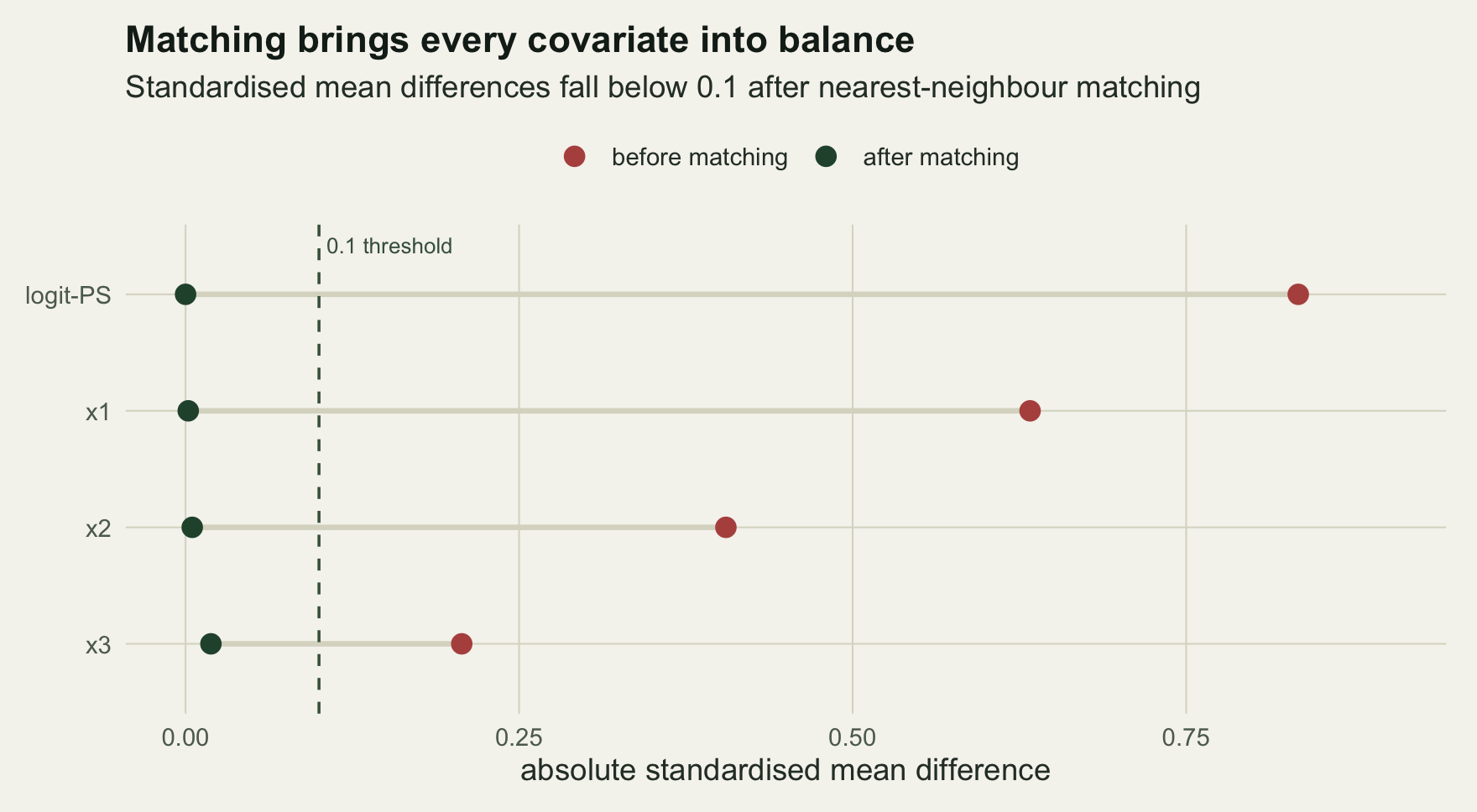
image-alt: "A Love plot with four rows labelled logit-PS, x1, x2 and x3, each a pale segment joining a dark green after-matching point to a brick red before-matching point. The before-matching points spread from about 0.21 to about 0.83 on an axis of absolute standardised mean difference; every after-matching point sits left of a dashed line annotated as the 0.1 threshold."
---
```{r}
#| label: setup
#| code-fold: true
#| code-summary: "Setup: packages, colours and plot theme"
#| results: hide
#| message: false
#| warning: false
knitr::opts_chunk$set(collapse = TRUE, comment = "#>", message = FALSE, warning = FALSE,
                      dev = "png", dpi = 110, fig.width = 8, fig.height = 4.4)
library(ggplot2)
te <- list(ink="#16241d", body="#2c3a31", forest="#275139", label="#46604a",
           paper="#f5f4ee", line="#dad9ca", faint="#5d6b61", grazed="#cda23f",
           mown="#2f8f63", abandoned="#b5534e", high="#1d5b4e", low="#c9b458")
theme_te <- function(base_size = 12) {
  theme_minimal(base_size = base_size) +
    theme(plot.background=element_rect(fill=te$paper,colour=NA),
          panel.background=element_rect(fill=te$paper,colour=NA),
          panel.grid.major=element_line(colour=te$line,linewidth=0.3),
          panel.grid.minor=element_blank(),
          axis.text=element_text(colour=te$faint), axis.title=element_text(colour=te$body),
          plot.title=element_text(colour=te$ink,face="bold"), plot.subtitle=element_text(colour=te$body),
          legend.text=element_text(colour=te$body), legend.title=element_text(colour=te$body),
          plot.margin=margin(10,12,10,10))
}
expit <- function(z) 1 / (1 + exp(-z))
```
The three previous tutorials removed confounding by modelling the outcome, weighting by the treatment probability, or combining the two. Matching takes a more direct line: for each treated unit find an untreated unit with the same propensity score, then compare their outcomes. Because it pairs treated units to comparable controls, matching estimates the effect of treatment on the treated (the ATT), which is often the quantity a manager cares about: what did the action do for the sites where it was actually taken?
## Matching on the logit of the propensity score
The [propensity score](../propensity-scores-and-ipw/) is the probability of treatment given the covariates. Two units with the same score have, on average, the same covariate distribution, so a treated and an untreated unit matched on the score are comparable. We match on the logit of the score rather than the score itself, because the logit spreads out the extremes and makes plain differences more even, which gives better matches near zero and one. The recipe is nearest neighbour: for each treated unit take the control with the closest logit score, optionally within a caliper (a maximum allowed distance) and either allowing a control to be reused (with replacement) or not.
```{r}
#| label: dgp
expit <- function(z) 1 / (1 + exp(-z))
pa <- c(a0=-0.3, a1=0.7, a2=0.5, a3=0.5)                 # propensity
pb <- c(b0=-0.4, bD=log(1.8), b1=0.6, b2=0.5, b3=0.5)    # outcome

gen <- function(n) {
  x1 <- rnorm(n); x2 <- rnorm(n); x3 <- rbinom(n, 1, 0.5)
  ps <- expit(pa["a0"] + pa["a1"]*x1 + pa["a2"]*x2 + pa["a3"]*x3)
  d  <- rbinom(n, 1, ps)
  py <- expit(pb["b0"] + pb["bD"]*d + pb["b1"]*x1 + pb["b2"]*x2 + pb["b3"]*x3)
  y  <- rbinom(n, 1, py)
  data.frame(y, d, x1, x2, x3)
}
true_att <- function(dat) {                              # E[Y(1) - Y(0) | D = 1]
  t <- dat$d == 1
  l1 <- pb["b0"]+pb["bD"]*1+pb["b1"]*dat$x1+pb["b2"]*dat$x2+pb["b3"]*dat$x3
  l0 <- pb["b0"]+pb["bD"]*0+pb["b1"]*dat$x1+pb["b2"]*dat$x2+pb["b3"]*dat$x3
  as.numeric(mean((expit(l1)-expit(l0))[t]))
}
```
```{r}
#| label: match-fns
match_repl <- function(lps, d, y, caliper=NULL) {        # nearest neighbour, with replacement
  it <- which(d==1); ic <- which(d==0)
  Dm <- abs(outer(lps[it], lps[ic], "-"))
  nn <- max.col(-Dm, ties.method="first")                # index of nearest control per treated
  md <- Dm[cbind(seq_along(it), nn)]
  keep <- if (is.null(caliper)) rep(TRUE, length(it)) else md <= caliper
  list(att=mean(y[it][keep]-y[ic][nn[keep]]), n_keep=sum(keep), n_t=length(it),
       t_idx=it[keep], c_idx=ic[nn[keep]])
}
match_norepl <- function(lps, d, y, caliper=NULL) {      # greedy, without replacement, high-PS first
  it <- which(d==1); ic <- which(d==0)
  ord <- it[order(lps[it], decreasing=TRUE)]
  avail <- rep(TRUE, length(ic)); tu <- cu <- integer(0)
  for (t in ord) {
    dd <- abs(lps[ic]-lps[t]); dd[!avail] <- Inf
    j <- which.min(dd)
    if (is.finite(dd[j]) && (is.null(caliper) || dd[j] <= caliper)) {
      avail[j] <- FALSE; tu <- c(tu, t); cu <- c(cu, ic[j])
    }
  }
  list(att=mean(y[tu]-y[cu]), n_keep=length(tu), n_t=length(it), t_idx=tu, c_idx=cu)
}
ipw_att <- function(e, d, y) {                           # ATT by weighting controls by e/(1-e)
  w <- e/(1-e)
  mean(y[d==1]) - sum(w[d==0]*y[d==0])/sum(w[d==0])
}
smd_treated <- function(x, ti, ci) (mean(x[ti]) - mean(x[ci])) / sd(x[ti])
```
## Fit and match
```{r}
#| label: data
set.seed(168)
n <- 2000
dat <- gen(n)
ps <- glm(d ~ x1 + x2 + x3, binomial, dat)
e <- fitted(ps); lps <- qlogis(e)
cal <- 0.2 * sd(lps) # standard caliper on the logit scale
TA <- true_att(dat)
c(n_treated = sum(dat$d), n_control = sum(1-dat$d),
overlap_low = max(min(e[dat$d==1]), min(e[dat$d==0])),
overlap_high = min(max(e[dat$d==1]), max(e[dat$d==0])), caliper = cal)
```
There are `r sum(dat$d)` treated and `r sum(1-dat$d)` control units, with propensities overlapping from about `r sprintf("%.2f", max(min(e[dat$d==1]), min(e[dat$d==0])))` to `r sprintf("%.2f", min(max(e[dat$d==1]), max(e[dat$d==0])))`. Now compute the naive contrast, three matched estimates and the weighting estimate.
```{r}
#| label: estimates
naive <- mean(dat$y[dat$d==1]) - mean(dat$y[dat$d==0])
mr <- match_repl(lps, dat$d, dat$y) # with replacement, no caliper
mrc <- match_repl(lps, dat$d, dat$y, cal) # with replacement, caliper
mn <- match_norepl(lps, dat$d, dat$y, cal) # without replacement, caliper
iw <- ipw_att(e, dat$d, dat$y)
data.frame(
estimator = c("naive (treated - all controls)","matching with replacement",
"matching with replacement + caliper","matching without replacement + caliper",
"IPW (ATT weights)"),
att = round(c(naive, mr$att, mrc$att, mn$att, iw), 4),
matched = c(sum(dat$d), mr$n_keep, mrc$n_keep, mn$n_keep, sum(dat$d)))
```
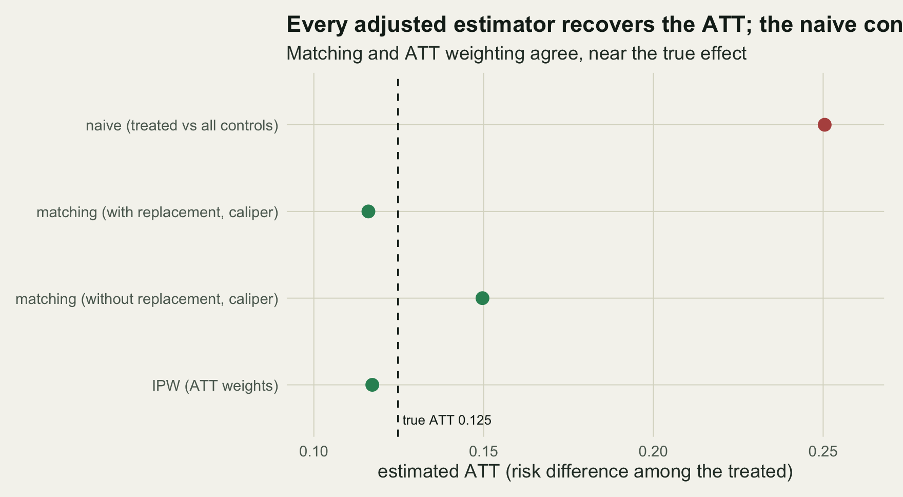
The true ATT on this sample is `r sprintf("%.3f", TA)`. The naive contrast, treated against all controls, is `r sprintf("%.3f", naive)`: treated sites have systematically higher covariate values, and the raw comparison blames the treatment for that. Matching with replacement inside a caliper gives `r sprintf("%.3f", mrc$att)`, and IPW on the same estimand gives `r sprintf("%.3f", iw)`. Matching without replacement plus a caliper is more demanding: it keeps only `r mn$n_keep` of the `r mr$n_t` treated units because each control can be used once and the high-propensity treated compete for the same scarce controls, so its estimate of `r sprintf("%.3f", mn$att)` now refers to a matchable subset rather than to all treated.
## The point of matching is balance
Matching earns its keep only if the matched controls actually resemble the treated. Standardised mean differences, the covariate mean gap divided by the treated standard deviation, make that checkable. Below 0.1 in absolute value is the usual target.
```{r}
#| label: balance
vars <- c("x1","x2","x3")
ti0 <- which(dat$d==1); ci0 <- which(dat$d==0)
bal <- data.frame(
variable = c(vars, "logit-PS"),
before = c(sapply(vars, function(v) smd_treated(dat[[v]], ti0, ci0)), smd_treated(lps, ti0, ci0)),
after = c(sapply(vars, function(v) smd_treated(dat[[v]], mrc$t_idx, mrc$c_idx)),
smd_treated(lps, mrc$t_idx, mrc$c_idx)))
round(bal[, -1], 3) -> bal[, -1]; bal
```
Before matching the imbalance is severe, up to `r sprintf("%.2f", max(abs(bal$before)))` standardised units on the logit score. After matching the largest imbalance is `r sprintf("%.2f", max(abs(bal$after)))` standardised units, under the 0.1 target. The Love plot shows the collapse at a glance.
```{r}
#| label: fig-love
#| fig-cap: "Absolute standardised mean differences for the three covariates and the logit propensity score, before and after nearest-neighbour matching with a caliper. Every value drops below the 0.1 threshold once treated units are compared with their matched controls."
#| fig-alt: "A dot plot with four rows. Before matching the values range up to 0.83; after matching all four sit to the left of a dashed line at 0.1."
lp <- rbind(data.frame(var=bal$variable, smd=abs(bal$before), when="before matching"),
            data.frame(var=bal$variable, smd=abs(bal$after),  when="after matching"))
lp$var  <- factor(lp$var, levels=rev(c("logit-PS","x1","x2","x3")))
lp$when <- factor(lp$when, levels=c("before matching","after matching"))
ggplot(lp, aes(smd, var)) +
  geom_line(aes(group=var), colour=te$line, linewidth=1) +
  geom_vline(xintercept=0.1, linetype="dashed", colour=te$label) +
  geom_point(aes(colour=when), size=3.2) +
  annotate("text", x=0.1, y=4.42, label="0.1 threshold", hjust=-0.06, size=3, colour=te$label) +
  scale_colour_manual(values=c("before matching"=te$abandoned, "after matching"=te$forest), name=NULL) +
  scale_x_continuous(limits=c(0, 0.9)) +
  labs(x="absolute standardised mean difference", y=NULL,
       title="Matching brings every covariate into balance",
       subtitle="Standardised mean differences fall below 0.1 after nearest-neighbour matching") +
  theme_te() + theme(legend.position="top")
```
## Matching against weighting
Matching and ATT weighting target the same estimand and, here, agree. They differ in what they do with the data: matching discards controls that are far from any treated unit, keeping an interpretable paired sample, while weighting keeps every control but down-weights the far ones. The comparison plot places the estimators against the true effect.
```{r}
#| label: fig-att
#| fig-cap: "Estimated ATT from each method against the true value, marked by the dashed line. The naive estimate sits well to the right of it, and the estimate from matching without replacement sits between the line and the naive point."
#| fig-alt: "A dot plot of four estimates on a horizontal axis, with a dashed vertical line at the true ATT near 0.12 and a label naming it. The naive estimate near 0.25 sits far to the right of that line. The estimate from matching with replacement and the weighting estimate both sit just to the left of the line, and the estimate from matching without replacement sits to the right of it, between those two and the naive point."
lab <- c("naive (treated - all controls)"="naive (treated vs all controls)",
         "matching with replacement + caliper"="matching (with replacement, caliper)",
         "matching without replacement + caliper"="matching (without replacement, caliper)",
         "IPW (ATT weights)"="IPW (ATT weights)")
es <- data.frame(estimator=names(lab),
                 att=c(naive, mrc$att, mn$att, iw))
es$label <- factor(lab[es$estimator],
  levels=rev(c("naive (treated vs all controls)","matching (with replacement, caliper)",
               "matching (without replacement, caliper)","IPW (ATT weights)")))
es$kind <- ifelse(es$estimator=="naive (treated - all controls)", "naive", "adjusted")
ggplot(es, aes(att, label, colour=kind)) +
  geom_vline(xintercept=TA, linetype="dashed", colour=te$ink) +
  geom_point(size=3.4) +
  annotate("text", x=TA, y=0.6, label=paste0("true ATT ", sprintf('%.3f', TA)),
           hjust=-0.05, size=3, colour=te$ink) +
  scale_colour_manual(values=c(naive=te$abandoned, adjusted=te$mown), guide="none") +
  scale_x_continuous(limits=c(0.10, 0.26)) +
  labs(x="estimated ATT (risk difference among the treated)", y=NULL,
       title="Estimated ATT by method, against the true value",
       subtitle="Naive contrast, two matching estimates and ATT weighting; the true ATT is marked") +
  theme_te() +
  theme(plot.title.position = "plot")
```
## It is unbiased across datasets
Repeating the with-replacement caliper match over many datasets confirms that matching is essentially unbiased for the ATT, as is weighting, while the naive contrast is not.
```{r}
#| label: mc
set.seed(16800)
nsim <- 500
En <- Em <- Ei <- tr <- numeric(nsim); frac <- numeric(nsim)
for (s in 1:nsim) {
ds <- gen(n); tr[s] <- true_att(ds)
p <- glm(d ~ x1 + x2 + x3, binomial, ds); ee <- fitted(p); ll <- qlogis(ee)
En[s] <- mean(ds$y[ds$d==1]) - mean(ds$y[ds$d==0])
mm <- match_repl(ll, ds$d, ds$y, 0.2*sd(ll)); Em[s] <- mm$att; frac[s] <- mm$n_keep/sum(ds$d)
Ei[s] <- ipw_att(ee, ds$d, ds$y)
}
mt <- mean(tr)
data.frame(estimator = c("naive","matching (repl + caliper)","IPW (ATT)"),
mean = round(c(mean(En), mean(Em), mean(Ei)), 4),
bias = round(c(mean(En), mean(Em), mean(Ei)) - mt, 4),
sd = round(c(sd(En), sd(Em), sd(Ei)), 4))
```
Over `r nsim` datasets the mean true ATT is `r sprintf("%.3f", mt)`, and the caliper retains `r sprintf("%.1f%%", 100*mean(frac))` of treated units on average. Matching carries a bias of `r sprintf("%+.4f", mean(Em)-mt)` and weighting `r sprintf("%+.4f", mean(Ei)-mt)`, both negligible, against `r sprintf("%+.3f", mean(En)-mt)` for the naive contrast. Weighting is tighter (standard deviation `r sprintf("%.3f", sd(Ei))` against `r sprintf("%.3f", sd(Em))`) because it uses every control, whereas one-to-one matching throws information away.
## What matching does and does not fix
Matching removes imbalance only on the covariates you put in the score, and only where treated and control propensities overlap. Units with no comparable partner are dropped, which is honest but changes the estimand to the matchable treated, as the without-replacement fit above made visible. Balance on the propensity score does not guarantee balance on a covariate you left out or on an interaction, so the standardised mean differences are a diagnostic to report, not a formality. Nearest neighbour is only the simplest scheme; optimal, full, many-to-one and kernel matching trade bias against variance differently. Finally the pairing itself should enter the standard error: the simple pair difference used here understates uncertainty a little, and matched-pair or bootstrap standard errors are the usual fix.
## References
Rosenbaum P, Rubin D 1983. Biometrika 70(1):41-55 (10.1093/biomet/70.1.41).
Stuart E 2010. Statistical Science 25(1):1-21 (10.1214/09-STS313).
Ho D, Imai K, King G, Stuart E 2007. Political Analysis 15(3):199-236 (10.1093/pan/mpl013).
Austin P 2011. Multivariate Behavioral Research 46(3):399-424 (10.1080/00273171.2011.568786).
Larsen A, Meng K, Kendall B 2019. Methods in Ecology and Evolution 10(7):924-934 (10.1111/2041-210X.13190).
Arif S, MacNeil M 2022. Ecosphere 13(4):e4009 (10.1002/ecs2.4009).
Hernan M, Robins J 2020. Causal Inference: What If. Chapman and Hall/CRC (ISBN 978-1-4200-7616-5).
## Related tutorials
- [Propensity scores and inverse-probability weighting](../propensity-scores-and-ipw/)
- [Doubly robust estimation with AIPW](../doubly-robust-estimation-aipw/)
- [G-computation and standardisation](../g-computation-and-standardisation/)
- [Confounding and backdoor adjustment](../confounding-and-backdoor-adjustment/)