---
title: "Doubly robust estimation with AIPW"
description: "Augmented inverse-probability weighting is doubly robust: the causal effect stays consistent when either the propensity or the outcome model is right."
date: "2026-05-26 12:00"
categories: [causal inference, R, ecology tutorial]
image: thumbnail.png
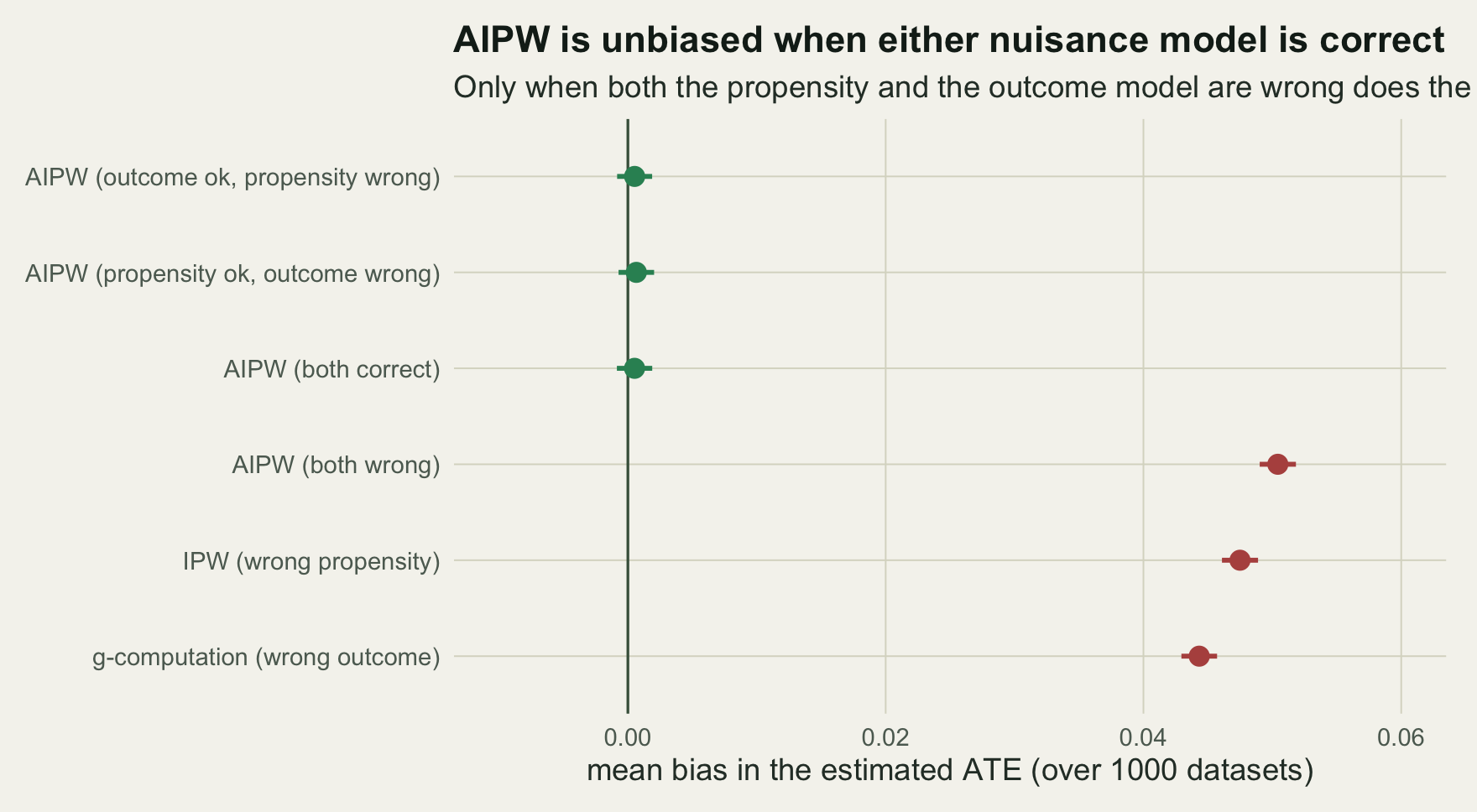
image-alt: "Dot and interval chart of mean bias in the estimated ATE over 1000 datasets for six estimators: the three AIPW rows with at least one correct nuisance model sit on the zero line, while AIPW with both models wrong, IPW with a wrong propensity and g-computation with a wrong outcome all sit just past the 0.04 tick."
---
```{r}
#| label: setup
#| code-fold: true
#| code-summary: "Setup: packages, colours and plot theme"
#| results: hide
#| message: false
#| warning: false
knitr::opts_chunk$set(collapse = TRUE, comment = "#>", message = FALSE, warning = FALSE,
                      dev = "png", dpi = 110, fig.width = 8, fig.height = 4.4)
library(ggplot2)
te <- list(ink="#16241d", body="#2c3a31", forest="#275139", label="#46604a",
           paper="#f5f4ee", line="#dad9ca", faint="#5d6b61", grazed="#cda23f",
           mown="#2f8f63", abandoned="#b5534e", high="#1d5b4e", low="#c9b458")
theme_te <- function(base_size = 12) {
  theme_minimal(base_size = base_size) +
    theme(plot.background=element_rect(fill=te$paper,colour=NA),
          panel.background=element_rect(fill=te$paper,colour=NA),
          panel.grid.major=element_line(colour=te$line,linewidth=0.3),
          panel.grid.minor=element_blank(),
          axis.text=element_text(colour=te$faint), axis.title=element_text(colour=te$body),
          plot.title=element_text(colour=te$ink,face="bold"), plot.subtitle=element_text(colour=te$body),
          legend.text=element_text(colour=te$body), legend.title=element_text(colour=te$body),
          plot.margin=margin(10,12,10,10))
}
expit <- function(z) 1 / (1 + exp(-z))
```
The two previous tutorials each rely on getting one model right. [Inverse-probability weighting](../propensity-scores-and-ipw/) needs a correct model for the treatment; [standardisation](../g-computation-and-standardisation/) needs a correct model for the outcome. In practice you are rarely sure which of the two you can specify well. Augmented inverse-probability weighting, AIPW, combines them and buys a genuine insurance policy: it estimates the effect consistently if either the treatment model or the outcome model is correct, not necessarily both. That property is called double robustness.
## The estimator
Take the standardisation estimate of the mean outcome under treatment level `a`, which is the average of the fitted values `m_a`, and add a weighted correction built from the residuals. For the treated arm the correction reweights the residual `y - m_1` by the inverse propensity, and symmetrically for the control arm. The contrast of the two corrected means is the estimate. In one line per unit,
$$
\psi_i = \left[\frac{D_i\,(Y_i - m_1(X_i))}{\pi(X_i)} + m_1(X_i)\right] - \left[\frac{(1-D_i)\,(Y_i - m_0(X_i))}{1-\pi(X_i)} + m_0(X_i)\right],
$$
and the estimated average treatment effect is the mean of `psi` over the sample. Here `pi` is the fitted propensity and `m_1`, `m_0` are the outcome-model predictions with treatment set to one and to zero. If the outcome model is perfect, the residuals vanish in expectation and the estimate reduces to standardisation. If the propensity model is perfect, the weighted residual removes whatever bias a wrong outcome model leaves behind. Either way the bias cancels.
```{r}
#| label: dgp
expit <- function(z) 1 / (1 + exp(-z))
pa <- c(a0=-0.5, a1=0.6, a2=0.4, a3=0.5, aq=0.35)          # true propensity
pb <- c(b0=-0.6, bD=log(2), b1=0.7, b2=0.5, b3=0.6, bq=0.5) # true outcome

gen <- function(n) {
  x1 <- rnorm(n); x2 <- rnorm(n); x3 <- rbinom(n, 1, 0.5)
  ps <- expit(pa["a0"] + pa["a1"]*x1 + pa["a2"]*x2 + pa["a3"]*x3 + pa["aq"]*x1^2)
  d  <- rbinom(n, 1, ps)
  py <- expit(pb["b0"] + pb["bD"]*d + pb["b1"]*x1 + pb["b2"]*x2 + pb["b3"]*x3 + pb["bq"]*x1^2)
  y  <- rbinom(n, 1, py)
  data.frame(y, d, x1, x2, x3)
}
true_ate <- function(dat) {
  l1 <- pb["b0"]+pb["bD"]*1+pb["b1"]*dat$x1+pb["b2"]*dat$x2+pb["b3"]*dat$x3+pb["bq"]*dat$x1^2
  l0 <- pb["b0"]+pb["bD"]*0+pb["b1"]*dat$x1+pb["b2"]*dat$x2+pb["b3"]*dat$x3+pb["bq"]*dat$x1^2
  as.numeric(mean(expit(l1)) - mean(expit(l0)))
}
```
Both the propensity and the outcome truly depend on `x1` squared. A model with only linear terms is therefore misspecified, which lets us switch each nuisance model between correct and wrong by including or dropping the square.
```{r}
#| label: estimators
gcomp <- function(om, dat)
  mean(predict(om, transform(dat, d=1), type="response")) -
  mean(predict(om, transform(dat, d=0), type="response"))

ipw <- function(pm, dat) {                          # normalised (Hajek) ATE
  e <- predict(pm, type="response"); d <- dat$d; y <- dat$y
  sum((d/e)*y)/sum(d/e) - sum(((1-d)/(1-e))*y)/sum((1-d)/(1-e))
}
aipw <- function(pm, om, dat) {
  e  <- predict(pm, type="response"); d <- dat$d; y <- dat$y
  m1 <- predict(om, transform(dat, d=1), type="response")
  m0 <- predict(om, transform(dat, d=0), type="response")
  psi <- (d*(y-m1)/e + m1) - ((1-d)*(y-m0)/(1-e) + m0)
  list(ate = mean(psi), se = sd(psi)/sqrt(length(psi)))
}
fit_all <- function(dat) list(
  om_c = glm(y ~ d + x1 + x2 + x3 + I(x1^2), binomial, dat),   # correct outcome
  om_w = glm(y ~ d + x1 + x2 + x3,           binomial, dat),   # wrong outcome
  pm_c = glm(d ~ x1 + x2 + x3 + I(x1^2),      binomial, dat),  # correct propensity
  pm_w = glm(d ~ x1 + x2 + x3,                binomial, dat))  # wrong propensity
```
## One dataset
Fit all four nuisance models, then read off standardisation, weighting and AIPW under every combination of correct and wrong.
```{r}
#| label: estimates
set.seed(167)
n <- 2000
dat <- gen(n)
f <- fit_all(dat)
e_c <- predict(f$pm_c, type="response")
TA <- true_ate(dat)
g_c <- gcomp(f$om_c, dat); g_w <- gcomp(f$om_w, dat)
i_c <- ipw(f$pm_c, dat); i_w <- ipw(f$pm_w, dat)
a_cc <- aipw(f$pm_c, f$om_c, dat); a_cw <- aipw(f$pm_c, f$om_w, dat)
a_wc <- aipw(f$pm_w, f$om_c, dat); a_ww <- aipw(f$pm_w, f$om_w, dat)
data.frame(
estimator = c("g-comp correct","g-comp wrong","IPW correct","IPW wrong",
"AIPW ok/ok","AIPW ok/wrong","AIPW wrong/ok","AIPW wrong/wrong"),
estimate = round(c(g_c,g_w,i_c,i_w,a_cc$ate,a_cw$ate,a_wc$ate,a_ww$ate), 4),
error = round(c(g_c,g_w,i_c,i_w,a_cc$ate,a_cw$ate,a_wc$ate,a_ww$ate) - TA, 4))
```
The true effect on this sample is a risk difference of `r sprintf("%.3f", TA)`. Standardisation with the wrong outcome model gives `r sprintf("%.3f", g_w)` and weighting with the wrong propensity gives `r sprintf("%.3f", i_w)`. AIPW gives `r sprintf("%.3f", a_cc$ate)` with both models correct, `r sprintf("%.3f", a_cw$ate)` with only the propensity correct, `r sprintf("%.3f", a_wc$ate)` with only the outcome correct, and `r sprintf("%.3f", a_ww$ate)` with both wrong. One dataset is suggestive rather than conclusive, so repeat the whole thing many times.
```{r}
#| label: mc
set.seed(16700)
nsim <- 1000
cols <- c("gc_w","ipw_w","aipw_cc","aipw_cw","aipw_wc","aipw_ww")
E <- matrix(NA_real_, nsim, length(cols), dimnames = list(NULL, cols))
tr <- numeric(nsim); cov_cc <- cov_cw <- cov_wc <- 0L
for (s in 1:nsim) {
ds <- gen(n); ta <- true_ate(ds); tr[s] <- ta
ff <- fit_all(ds)
E[s,"gc_w"] <- gcomp(ff$om_w, ds)
E[s,"ipw_w"] <- ipw(ff$pm_w, ds)
acc <- aipw(ff$pm_c, ff$om_c, ds); E[s,"aipw_cc"] <- acc$ate
acw <- aipw(ff$pm_c, ff$om_w, ds); E[s,"aipw_cw"] <- acw$ate
awc <- aipw(ff$pm_w, ff$om_c, ds); E[s,"aipw_wc"] <- awc$ate
E[s,"aipw_ww"] <- aipw(ff$pm_w, ff$om_w, ds)$ate
if (ta >= acc$ate-1.96*acc$se && ta <= acc$ate+1.96*acc$se) cov_cc <- cov_cc+1L
if (ta >= acw$ate-1.96*acw$se && ta <= acw$ate+1.96*acw$se) cov_cw <- cov_cw+1L
if (ta >= awc$ate-1.96*awc$se && ta <= awc$ate+1.96*awc$se) cov_wc <- cov_wc+1L
}
mtruth <- mean(tr)
bias <- colMeans(E) - mtruth
round(rbind(mean = colMeans(E), bias = bias, sd = apply(E, 2, sd)), 4)
```
Averaged over `r nsim` datasets, the mean true effect is `r sprintf("%.3f", mtruth)`. The two misspecified single-model estimators carry a bias of `r sprintf("%+.3f", bias["gc_w"])` (wrong outcome model) and `r sprintf("%+.3f", bias["ipw_w"])` (wrong propensity). Every AIPW variant with one correct model is effectively unbiased: `r sprintf("%+.4f", bias["aipw_cc"])`, `r sprintf("%+.4f", bias["aipw_cw"])` and `r sprintf("%+.4f", bias["aipw_wc"])`. The one AIPW that fails is the one with both models wrong, at `r sprintf("%+.3f", bias["aipw_ww"])`.
```{r}
#| label: fig-bias
#| fig-cap: "Mean bias in the estimated average treatment effect over 1000 datasets, with a tight Monte Carlo interval. AIPW is centred on zero whenever at least one nuisance model is correct; the bias returns only when both are wrong, matching the two misspecified single-model estimators."
#| fig-alt: "A horizontal interval plot. Three AIPW variants with at least one correct model sit on the zero line. Standardisation with a wrong outcome model, weighting with a wrong propensity, and AIPW with both wrong sit near a bias of 0.05."
lab <- c(gc_w="g-computation (wrong outcome)", ipw_w="IPW (wrong propensity)",
         aipw_ww="AIPW (both wrong)", aipw_cc="AIPW (both correct)",
         aipw_cw="AIPW (propensity ok, outcome wrong)", aipw_wc="AIPW (outcome ok, propensity wrong)")
ord <- c("gc_w","ipw_w","aipw_ww","aipw_cc","aipw_cw","aipw_wc")
b <- data.frame(key=ord, bias=bias[ord], se=apply(E,2,sd)[ord]/sqrt(nsim))
b$label <- factor(lab[ord], levels=lab[ord])
b$kind  <- ifelse(abs(b$bias) < 0.01, "consistent", "biased")
p_bias <- ggplot(b, aes(bias, label, colour=kind)) +
  geom_vline(xintercept=0, colour=te$label, linewidth=0.5) +
  geom_pointrange(aes(xmin=bias-1.96*se, xmax=bias+1.96*se), linewidth=0.9, size=0.6) +
  scale_colour_manual(values=c(consistent=te$mown, biased=te$abandoned), guide="none") +
  scale_x_continuous(limits=c(-0.01, 0.06)) +
  labs(x="mean bias in the estimated ATE (over 1000 datasets)", y=NULL,
       title="AIPW stays centred when either nuisance model is correct",
       subtitle="The bias returns only when both nuisance models are wrong") +
  theme_te() + theme(plot.title.position = "plot")
p_bias
```
```{r}
#| label: thumb
#| include: false
ggsave("thumbnail.png",
p_bias + labs(title = NULL, subtitle = NULL) +
theme(axis.title.x = element_text(size = 9.5),
plot.margin = margin(8, 14, 8, 8)),
width = 7.5, height = 5.4, dpi = 100, bg = te$paper)
```
## Why one correct model suffices
The augmentation term is a product of two errors: the treatment-model error and the outcome-model error. If the propensity is right, the inverse-probability weighting makes the outcome-model error average to zero, so a wrong outcome model does no harm. If the outcome model is right, its residuals already have mean zero within covariate strata, so a wrong propensity multiplies something that is already centred. The bias survives only when both pieces are wrong at once, because then neither factor is there to cancel it. That is the whole content of double robustness.
## Uncertainty and coverage
Because AIPW is an average of the per-unit quantity `psi`, its standard error is just the standard deviation of `psi` divided by the square root of the sample size, the influence-function estimator. It performs well here.
```{r}
#| label: coverage
c(both_correct = cov_cc, ps_ok_out_wrong = cov_cw, out_ok_ps_wrong = cov_wc) / nsim
```
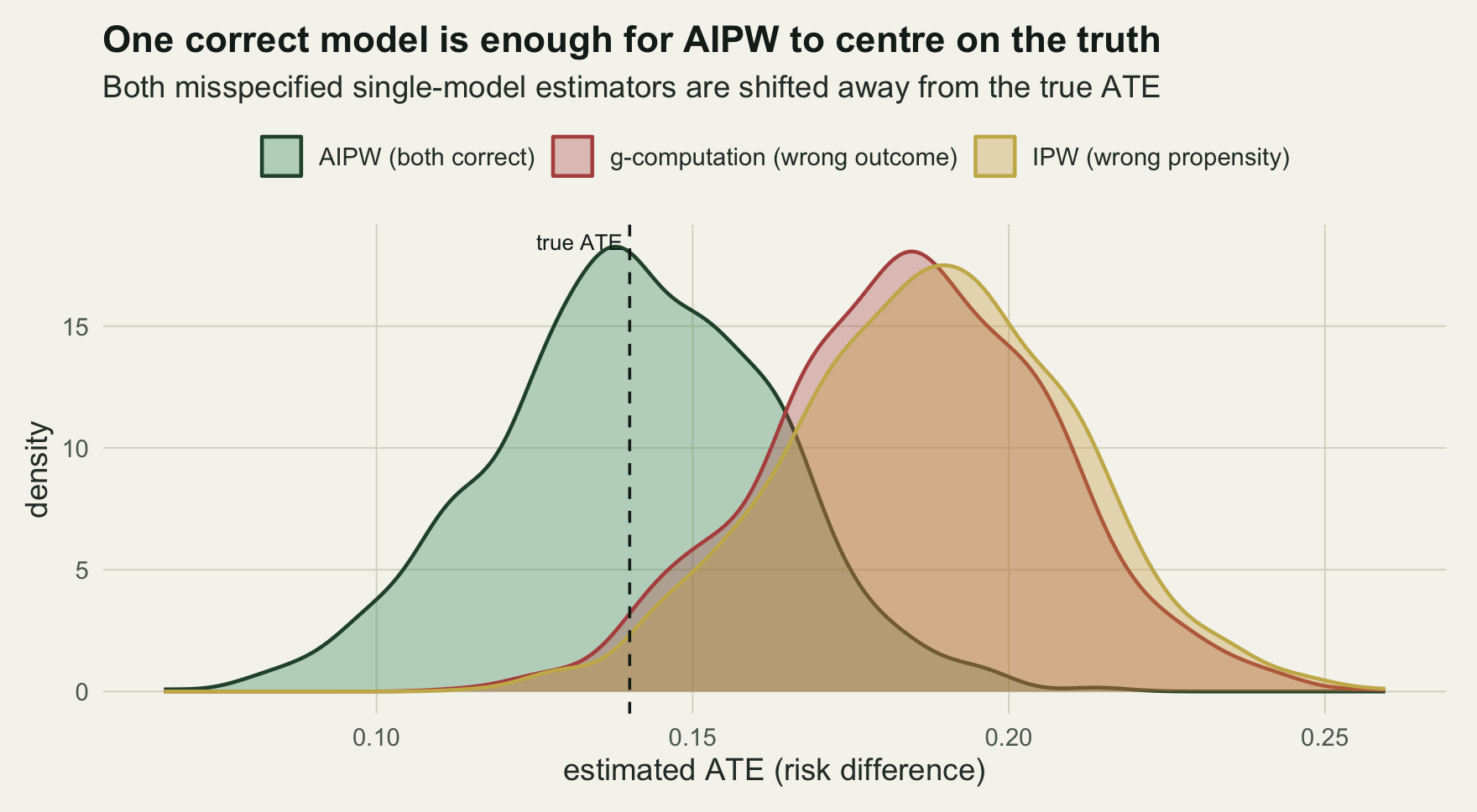
Interval coverage is close to the nominal 95%: `r sprintf("%.1f%%", 100*cov_cc/nsim)` with both models correct, `r sprintf("%.1f%%", 100*cov_cw/nsim)` with only the propensity correct, and `r sprintf("%.1f%%", 100*cov_wc/nsim)` with only the outcome correct. The plug-in standard error stays honest even when one nuisance model is misspecified.
```{r}
#| label: fig-dist
#| fig-cap: "Sampling distribution of the estimated average treatment effect over 1000 datasets. AIPW with both models correct is centred on the true effect, while both misspecified single-model estimators are shifted to the right."
#| fig-alt: "Three overlaid density curves. The AIPW curve is centred on a dashed line at the true effect near 0.14. The wrong-outcome standardisation curve and the wrong-propensity weighting curve are separate peaks to the right, near 0.19."
dd <- rbind(data.frame(ate=E[,"aipw_cc"], est="AIPW (both correct)"),
            data.frame(ate=E[,"gc_w"],    est="g-computation (wrong outcome)"),
            data.frame(ate=E[,"ipw_w"],   est="IPW (wrong propensity)"))
dd$est <- factor(dd$est, levels=c("AIPW (both correct)","g-computation (wrong outcome)","IPW (wrong propensity)"))
ggplot(dd, aes(ate, fill=est, colour=est)) +
  geom_density(alpha=0.32, linewidth=0.7) +
  geom_vline(xintercept=mtruth, linetype="dashed", colour=te$ink) +
  annotate("text", x=mtruth, y=Inf, label="true ATE", vjust=1.6, hjust=1.08, size=3, colour=te$ink) +
  scale_y_continuous(expand=expansion(mult=c(0.05, 0.15))) +
  scale_fill_manual(values=c("AIPW (both correct)"=te$mown,
                             "g-computation (wrong outcome)"=te$abandoned,
                             "IPW (wrong propensity)"=te$grazed), name=NULL) +
  scale_colour_manual(values=c("AIPW (both correct)"=te$forest,
                               "g-computation (wrong outcome)"=te$abandoned,
                               "IPW (wrong propensity)"=te$low), name=NULL) +
  labs(x="estimated ATE (risk difference)", y="density",
       title="One correct model is enough for AIPW to centre on the truth",
       subtitle="Both misspecified single-model estimators are shifted away from the true ATE") +
  theme_te() + theme(legend.position="top")
```
## What it does not buy you
Double robustness is insurance against one wrong model, not against both: the both-wrong AIPW above is as biased as the misspecified single-model fits, so the property is not a substitute for thinking about either model. It also does not repair poor overlap. The correct propensities in this sample run from `r sprintf("%.3f", min(e_c))` to `r sprintf("%.3f", max(e_c))`, so a few units carry large weights. Those weights enter the weighting estimator and AIPW, which both divide by the fitted propensity. When both nuisance models are correct AIPW is also efficient, reaching the smallest possible large-sample variance, which is a second reason to prefer it. Fitting the nuisance models with flexible machine learning brings its own subtlety and needs sample splitting (cross-fitting), the route taken by targeted learning and double machine learning, beyond the scope here.
## References
Robins J, Rotnitzky A, Zhao L 1994. Journal of the American Statistical Association 89(427):846-866 (10.2307/2290910).
Bang H, Robins J 2005. Biometrics 61(4):962-973 (10.1111/j.1541-0420.2005.00377.x).
Kang J, Schafer J 2007. Statistical Science 22(4):523-539 (10.1214/07-STS227).
Funk M, Westreich D, Wiesen C, Sturmer T, Brookhart M, Davidian M 2011. American Journal of Epidemiology 173(7):761-767 (10.1093/aje/kwq439).
Larsen A, Meng K, Kendall B 2019. Methods in Ecology and Evolution 10(7):924-934 (10.1111/2041-210X.13190).
Arif S, MacNeil M 2022. Ecosphere 13(4):e4009 (10.1002/ecs2.4009).
Hernan M, Robins J 2020. Causal Inference: What If. Chapman and Hall/CRC (ISBN 978-1-4200-7616-5).
## Related tutorials
- [G-computation and standardisation](../g-computation-and-standardisation/)
- [Propensity scores and inverse-probability weighting](../propensity-scores-and-ipw/)
- [Propensity score matching](../propensity-score-matching/)
- [Sensitivity to unmeasured confounding](../sensitivity-to-unmeasured-confounding/)