Sensitivity to unmeasured confounding

How strong must an unmeasured confounder be to overturn a causal finding? The E-value and Rosenbaum bounds in base R, calibrated against a known confounder.

Every method in this series so far, adjustment, weighting, matching and AIPW, rests on one assumption the data can never confirm: that you have measured every common cause of treatment and outcome. Sensitivity analysis accepts that you might not have, and asks the next best question. How strong would an unmeasured confounder need to be, in its associations with both treatment and outcome, before it could overturn the finding? This closing tutorial builds two answers in base R: the E-value for an effect estimate, and Rosenbaum bounds for a matched test, and calibrates each against a confounder whose strength we actually know.

A finding with a confounder left out

There is a measured covariate x and an unmeasured binary confounder u that drives both treatment and outcome. We fit a model adjusting for x only, exactly as an analyst who never recorded u would, so the estimate carries whatever confounding u leaves behind.

expit <- function(z) 1 / (1 + exp(-z))
pa <- c(a0=-0.2, ax=0.5, au=log(1.7))                # treatment: u odds ratio 1.7
pb <- c(b0=-0.8, bD=log(1.8), bx=0.5, bu=log(2.0))   # outcome: u odds ratio 2.0, true effect 1.8

gen <- function(n) {
  x <- rnorm(n); u <- rbinom(n, 1, 0.5)
  d <- rbinom(n, 1, expit(pa["a0"] + pa["ax"]*x + pa["au"]*u))
  y <- rbinom(n, 1, expit(pb["b0"] + pb["bD"]*d + pb["bx"]*x + pb["bu"]*u))
  data.frame(y, d, x, u)
}
true_rr <- function(dat) {                           # true marginal risk ratio (over x and u)
  l1 <- pb["b0"]+pb["bD"]*1+pb["bx"]*dat$x+pb["bu"]*dat$u
  l0 <- pb["b0"]+pb["bD"]*0+pb["bx"]*dat$x+pb["bu"]*dat$u
  as.numeric(mean(expit(l1))/mean(expit(l0)))
}
gcomp_rr <- function(model, dat) {                   # marginal RR by standardisation
  mean(predict(model, transform(dat, d=1), type="response")) /
  mean(predict(model, transform(dat, d=0), type="response"))
}
evalue      <- function(rr) { r <- ifelse(rr < 1, 1/rr, rr); as.numeric(r + sqrt(r*(r-1))) }
bias_factor <- function(rud, ruy) as.numeric(rud*ruy/(rud+ruy-1))

set.seed(169)
n <- 3000
dat <- gen(n)
m_x <- glm(y ~ d + x, binomial, dat)                 # adjusts for x only; u is unmeasured
RR  <- gcomp_rr(m_x, dat)
set.seed(1690); B <- 500; bs <- numeric(B)
for (b in 1:B) { idx <- sample.int(n, n, TRUE); db <- dat[idx, ]
  bs[b] <- gcomp_rr(glm(y ~ d + x, binomial, db), db) }
ci <- quantile(bs, c(.025, .975))
TR <- true_rr(dat)
c(true_RR = TR, observed_RR = RR, lower = ci[[1]], upper = ci[[2]])
#>     true_RR observed_RR       lower       upper 
#>    1.331564    1.498930    1.379351    1.615728

The true marginal risk ratio is 1.33, but with u left out the analysis reports 1.50 (95% CI 1.38 to 1.62), inflated by the residual confounding. An analyst looking only at this output sees a clear positive effect and has no way to know how much of it is real.

The E-value

The E-value is the smallest association, on the risk-ratio scale, that an unmeasured confounder would need with both the treatment and the outcome, above and beyond the measured covariates, to reduce the observed effect to the null (Ding and VanderWeele 2016; VanderWeele and Ding 2017). For an observed risk ratio above one it has a closed form.

ev_pt <- evalue(RR)
ev_ci <- evalue(ci[[1]])                             # applied to the confidence limit nearest the null
c(evalue_point = ev_pt, evalue_ci = ev_ci)
#> evalue_point    evalue_ci 
#>     2.363719     2.102716

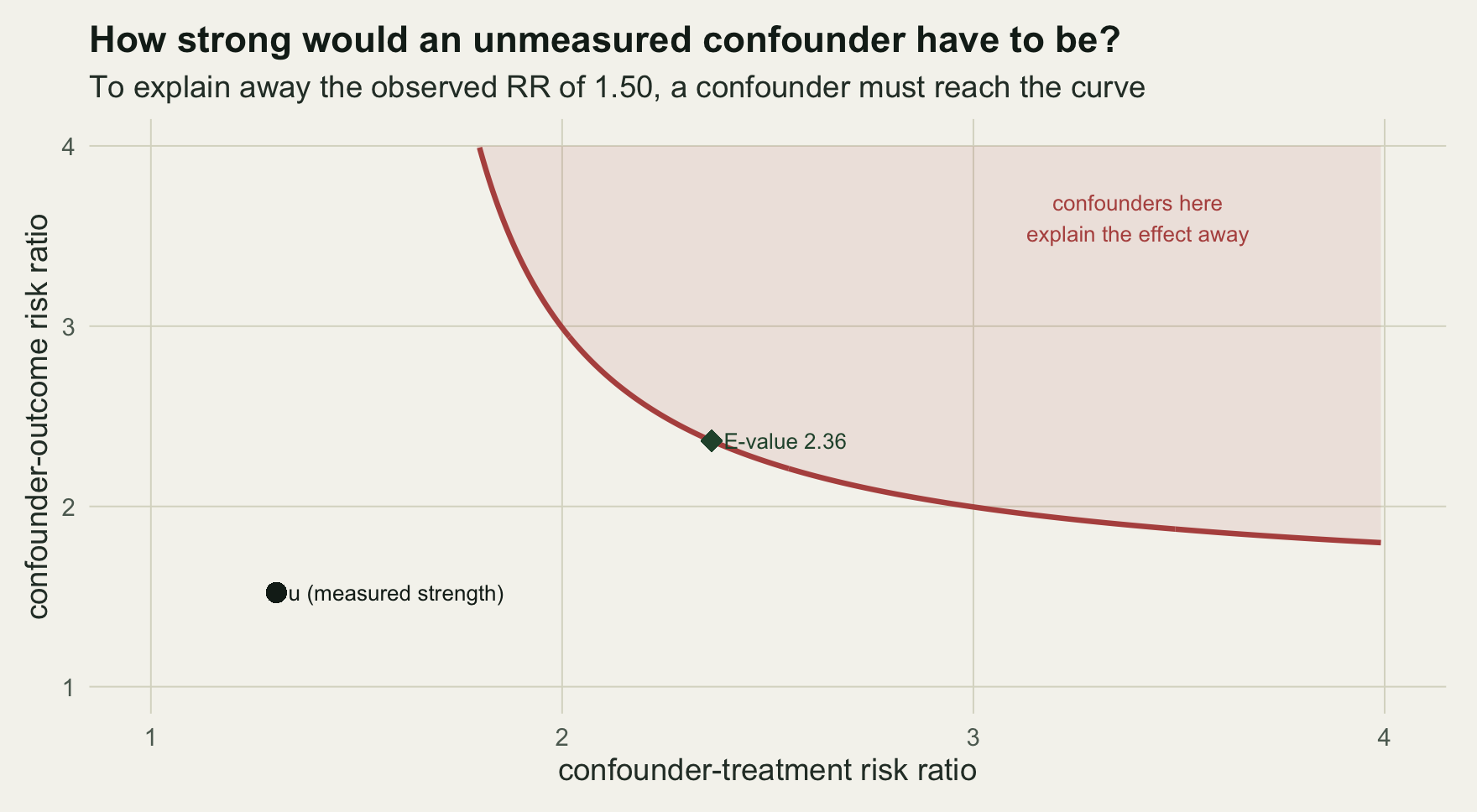
The point estimate has an E-value of 2.36: only a confounder associated with both treatment and outcome by a risk ratio of at least 2.36 each could account for the whole of the observed effect. Weaker confounding cannot. Applied to the confidence limit nearest the null, the E-value is 2.10, the strength needed merely to push the interval across one. The contour below traces every pair of associations that would just explain the estimate away.

E <- ev_pt
a <- seq(RR+0.002, 4, 0.01); bb <- RR*(a-1)/(a-RR)
curve <- rbind(data.frame(rud=a, ruy=bb), data.frame(rud=bb, ruy=a))
curve <- curve[curve$rud<=4 & curve$ruy<=4 & curve$ruy>=1 & curve$rud>=1, ]
RUD <- mean(dat$d[dat$u==1]) / mean(dat$d[dat$u==0])
RUY <- max(sapply(0:1, function(dd)
  mean(dat$y[dat$u==1 & dat$d==dd]) / mean(dat$y[dat$u==0 & dat$d==dd])))
ggplot(curve[order(curve$rud), ], aes(rud, ruy)) +
  geom_ribbon(data=data.frame(x=a, lo=pmin(bb,4)), aes(x=x, ymin=lo, ymax=4),
              inherit.aes=FALSE, fill=te$abandoned, alpha=0.10) +
  geom_line(linewidth=1, colour=te$abandoned) +
  geom_point(aes(x=E, y=E), colour=te$forest, size=3.6, shape=18) +
  geom_point(aes(x=RUD, y=RUY), colour=te$ink, size=3) +
  annotate("text", x=E, y=E, label=paste0("  E-value ", sprintf('%.2f', E)), hjust=0, size=3, colour=te$forest) +
  annotate("text", x=RUD, y=RUY, label="  u (measured strength)", hjust=0, size=3, colour=te$ink) +
  annotate("text", x=3.4, y=3.6, label="confounders here\nexplain the effect away", size=3, colour=te$abandoned) +
  coord_cartesian(xlim=c(1,4), ylim=c(1,4)) +
  labs(x="confounder-treatment risk ratio", y="confounder-outcome risk ratio",
       title="How strong would an unmeasured confounder have to be?",
       subtitle=paste0("To explain away the observed RR of ", sprintf('%.2f', RR),
                       ", a confounder must reach the curve")) +
  theme_te()

Figure 1: Combinations of the confounder-treatment and confounder-outcome risk ratios that would explain away the observed effect. Anything on or beyond the curve suffices; the diamond marks the E-value, where the two associations are equal. The real confounder u sits well inside the safe region.

Calibrating against the real confounder

Because this is a simulation we can measure u and check the E-value against it. Its associations with treatment and outcome on the risk-ratio scale, and the bias factor they generate, tell us exactly how much u could distort the estimate.

BFu <- bias_factor(RUD, RUY)
c(RR_ud = RUD, RR_uy = RUY, bias_factor = BFu, observed_RR = RR)
#>       RR_ud       RR_uy bias_factor observed_RR 
#>    1.305236    1.522180    1.087221    1.498930
c(u_can_explain_point = BFu >= RR, u_reaches_evalue = (RUD >= ev_pt && RUY >= ev_pt))
#> u_can_explain_point    u_reaches_evalue 
#>               FALSE               FALSE

The confounder u has associations of 1.31 and 1.52, giving a bias factor of 1.09. That is below the observed risk ratio of 1.50, so u cannot pull the estimate to the null, and both of its associations fall short of the E-value of 2.36. The finding of a positive effect withstands a confounder as strong as u, which matches the ground truth: the real risk ratio is 1.33, still comfortably above one. The E-value did its job as a benchmark, and u sits below it.

Rosenbaum bounds for a matched test

A matched analysis invites a different sensitivity question. If we match on x and test the treatment effect with McNemar’s test on the discordant pairs, how much could two matched units differ in their true treatment odds, because of some unmeasured u, before the significant result could be an artefact of that hidden bias? The parameter is Rosenbaum’s Gamma: Gamma of one means matched units are equally likely to be treated, and larger values allow more hidden bias.

ps <- glm(d ~ x, binomial, dat); lps <- qlogis(fitted(ps))
it <- which(dat$d==1); ic <- which(dat$d==0)
ord <- it[order(lps[it], decreasing=TRUE)]; avail <- rep(TRUE, length(ic)); cal <- 0.2*sd(lps)
tp <- cp <- integer(0)
for (t in ord) { dd <- abs(lps[ic]-lps[t]); dd[!avail] <- Inf; j <- which.min(dd)
  if (is.finite(dd[j]) && dd[j] <= cal) { avail[j] <- FALSE; tp <- c(tp,t); cp <- c(cp,ic[j]) } }
bcnt <- sum(dat$y[tp]==1 & dat$y[cp]==0)              # pairs: treated has event, control does not
ccnt <- sum(dat$y[tp]==0 & dat$y[cp]==1)              # the reverse
m <- bcnt + ccnt
p_one <- pbinom(bcnt-1, m, 0.5, lower.tail=FALSE)     # McNemar, one sided, no hidden bias

p_upper <- function(g) pbinom(bcnt-1, m, g/(1+g), lower.tail=FALSE)   # worst-case p at bias g
gammas <- seq(1, 6, 0.01); pu <- sapply(gammas, p_upper)
gstar <- gammas[which(pu > 0.05)[1]]
c(pairs = length(tp), discordant = m, b = bcnt, c = ccnt, mcnemar_p = p_one, gamma_star = gstar)
#>        pairs   discordant            b            c    mcnemar_p   gamma_star 
#> 1.320000e+03 6.660000e+02 4.710000e+02 1.950000e+02 1.442492e-27 2.100000e+00

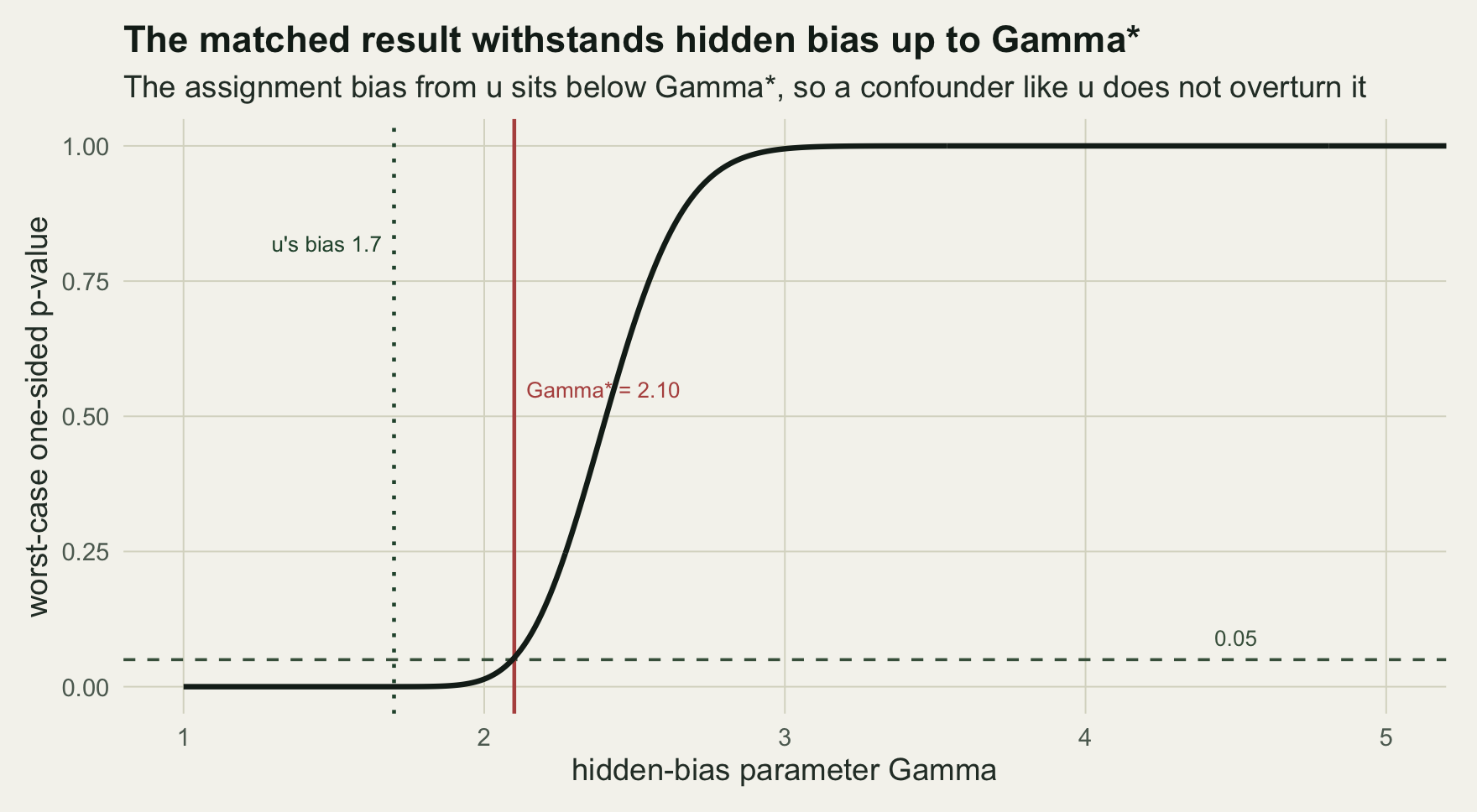
There are 1320 matched pairs, of which 666 are discordant: 471 favour the treated unit against 195 the other way, a result the McNemar test rejects decisively (p 1e-27) when there is no hidden bias. The sensitivity curve raises the bias steadily until the worst-case p-value crosses 0.05, which happens at Gamma of 2.10.

sens <- data.frame(gamma=gammas, p=pu)
ggplot(sens, aes(gamma, p)) +
  geom_hline(yintercept=0.05, linetype="dashed", colour=te$label) +
  geom_vline(xintercept=gstar, colour=te$abandoned, linewidth=0.7) +
  geom_vline(xintercept=exp(pa["au"]), colour=te$forest, linewidth=0.7, linetype="dotted") +
  geom_line(linewidth=1, colour=te$ink) +
  annotate("text", x=gstar, y=0.55, label=paste0("  Gamma* = ", sprintf('%.2f', gstar)), hjust=0, size=3, colour=te$abandoned) +
  annotate("text", x=exp(pa["au"]), y=0.82, label=paste0("u's bias ", sprintf('%.1f', exp(pa["au"])), "  "), hjust=1, size=3, colour=te$forest) +
  annotate("text", x=4.5, y=0.09, label="0.05", size=3, colour=te$label) +
  coord_cartesian(xlim=c(1,5), ylim=c(0,1)) +
  labs(x="hidden-bias parameter Gamma", y="worst-case one-sided p-value",
       title="The matched result withstands hidden bias up to Gamma*",
       subtitle="The assignment bias from u sits below Gamma*, so a confounder like u does not overturn it") +
  theme_te()

Figure 2: Worst-case one-sided p-value for the matched McNemar test as hidden bias grows. The result stays significant until Gamma reaches the value marked; the treatment-assignment bias generated by u lies to the left of that point, so a confounder like u does not overturn the finding.

The treatment-assignment odds ratio that u actually generates is 1.7, below Gamma of 2.10, so once again a confounder of u’s strength leaves the conclusion standing. The two analyses agree, though they measure different things: the E-value combines both arms of the confounding into a single joint strength, whereas Rosenbaum’s Gamma bounds only the assignment arm and takes the worst case over the outcome arm, which makes it the more cautious of the two.

set.seed(16900); nsim <- 300; eb <- tb <- numeric(nsim)
for (s in 1:nsim) { ds <- gen(n); tb[s] <- true_rr(ds)
  eb[s] <- gcomp_rr(glm(y ~ d + x, binomial, ds), ds) }
c(mean_true_RR = mean(tb), mean_observed_RR = mean(eb), bias = mean(eb) - mean(tb))
#>     mean_true_RR mean_observed_RR             bias 
#>       1.33723835       1.40085699       0.06361863

Across 300 datasets the estimate that omits u averages 1.40 against a true 1.34, an upward bias of 0.06. That gap is the residual confounding the sensitivity analyses were built to probe, and both correctly judged it too small to overturn the qualitative finding.

What sensitivity analysis can and cannot do

These tools do not detect confounding and do not prove its absence. They translate the untestable “no unmeasured confounding” into a magnitude you can argue about: an E-value of 2.36 or a Gamma of 2.10 is reassuring only if you can say, from subject knowledge, that no unmeasured confounder is that strongly related to both treatment and outcome once the measured covariates are accounted for. A large value is not a licence, and a small one is a warning that a modest confounder could change everything. They also speak only to confounding, saying nothing about selection bias or measurement error, and they pair naturally with the negative-control checks in checking causal assumptions, which look for confounding rather than bounding its effect.

References

Rosenbaum P, Rubin D 1983. Journal of the Royal Statistical Society Series B 45(2):212-218 (10.1111/j.2517-6161.1983.tb01242.x).

Ding P, VanderWeele T 2016. Epidemiology 27(3):368-377 (10.1097/EDE.0000000000000457).

VanderWeele T, Ding P 2017. Annals of Internal Medicine 167(4):268-274 (10.7326/M16-2607).

Cinelli C, Hazlett C 2020. Journal of the Royal Statistical Society Series B 82(1):39-67 (10.1111/rssb.12348).

Larsen A, Meng K, Kendall B 2019. Methods in Ecology and Evolution 10(7):924-934 (10.1111/2041-210X.13190).

Arif S, MacNeil M 2022. Ecosphere 13(5):e4009 (10.1002/ecs2.4009).

Hernan M, Robins J 2020. Causal Inference: What If. Chapman and Hall/CRC (ISBN 978-1-4200-7616-5).

Related tutorials

• Checking causal assumptions
• Propensity score matching
• Doubly robust estimation with AIPW
• Confounding and backdoor adjustment