library(ggplot2); library(dplyr); library(tidyr)
paper<-"#f5f4ee"; ink<-"#16241d"; body<-"#2c3a31"; forest<-"#275139"
sage<-"#93a87f"; line<-"#dad9ca"; faint<-"#5d6b61"; brick<-"#b5534e"
theme_te <- function(base=12) theme_minimal(base_size=base) +
  theme(plot.background=element_rect(fill=paper,colour=NA),
        panel.background=element_rect(fill=paper,colour=NA),
        panel.grid.major=element_line(colour=line,linewidth=0.3),
        panel.grid.minor=element_blank(),
        axis.text=element_text(colour=body), axis.title=element_text(colour=ink),
        plot.title=element_text(colour=ink,face="bold"),
plot.subtitle=element_text(colour=faint), legend.position="top")Propensity scores and IPW
R
causal inference
ecology tutorial
With many measured confounders, the propensity score balances the groups by weighting. Inverse-probability weighting, balance and overlap, built by hand in R.
When management is applied non-randomly across sites, the treated and untreated groups differ in the covariates that also drive the outcome, and a plain comparison confuses the treatment with those differences. Backdoor adjustment fixes this by putting the confounders in an outcome model (see confounding and backdoor adjustment). The propensity score offers a second route to the same target. It is the probability of being treated given the covariates, and it turns out to be a balancing score: among units with the same propensity, treated and untreated look alike in every covariate. Model the treatment once, use the score to weight or match, and the confounders balance out. This tutorial builds inverse-probability weighting by hand, shows the balance and overlap checks that make it credible, and shows the assumption that sinks it.
A confounded example
Four measured covariates drive both who gets treated and the outcome. The true treatment effect is 1.0.
set.seed(4165)
n <- 2000; tau <- 1.0
X1<-rnorm(n); X2<-rnorm(n); X3<-rnorm(n); X4<-rnorm(n)
D <- rbinom(n, 1, plogis(0.5*X1 + 0.7*X2 - 0.6*X3 + 0.8*X4))   # non-random treatment
Y <- tau*D + 1.0*X1 + 0.8*X2 + 1.2*X3 + 0.9*X4 + rnorm(n, 0, 1)
Of 2000 sites, 973 are treated and 1027 are not. Because the same covariates raise both the chance of treatment and the outcome, a plain difference in means is biased:
naive <- mean(Y[D==1]) - mean(Y[D==0])The unadjusted difference is 1.673, well above the true 1.0.
Propensity scores and weighting
Fit a logistic model for treatment given the covariates; its fitted values are the propensity scores. Weight each treated unit by the reciprocal of its score and each control by the reciprocal of one minus its score. In the weighted pseudo-population the covariates no longer predict treatment, and a weighted difference in means estimates the effect. A weighted regression of the outcome on treatment does exactly this.
ps <- glm(D ~ X1+X2+X3+X4, family=binomial)
e  <- fitted(ps)                       # propensity scores
w  <- D/e + (1-D)/(1-e)                 # inverse-probability weights
ipw <- coef(lm(Y ~ D, weights=w))["D"]
adj <- coef(lm(Y ~ D + X1+X2+X3+X4))["D"]   # outcome regression, for comparison
Weighting brings the estimate to 1.041, on the true 1.0. The outcome regression, correctly specified, lands at 1.000: two different mechanisms, one answer. The two can even be combined so that getting either the treatment model or the outcome model right is enough to strip out the confounding.
To attach honest uncertainty, resample the data and refit the whole pipeline, propensity model included, in each replicate.
set.seed(6165); B <- 600
bs <- t(sapply(1:B, function(b){
  i <- sample(n, n, replace=TRUE)
  d <- data.frame(Y=Y[i],D=D[i],X1=X1[i],X2=X2[i],X3=X3[i],X4=X4[i])
  nv <- mean(d$Y[d$D==1]) - mean(d$Y[d$D==0])
  ee <- fitted(glm(D~X1+X2+X3+X4, family=binomial, data=d))
  ww <- d$D/ee + (1-d$D)/(1-ee)
  c(naive=nv, ipw=unname(coef(lm(Y~D, weights=ww, data=d))["D"]))
}))
ci_naive <- quantile(bs[,"naive"], c(.025,.975))
ci_ipw   <- quantile(bs[,"ipw"],   c(.025,.975))
The naive interval, [1.48, 1.86], misses the truth entirely; the weighted interval, [0.90, 1.17], contains it.
Check the balance
The selling point of the propensity score is that the balance it buys is visible. For each covariate, the standardised mean difference between groups should shrink toward zero once weighted. Anything under about 0.1 is usually treated as balanced.
smd <- function(x, D, w=rep(1,length(x))){
  mt <- weighted.mean(x[D==1], w[D==1]); mc <- weighted.mean(x[D==0], w[D==0])
  sp <- sqrt((var(x[D==1]) + var(x[D==0]))/2); (mt - mc)/sp
}
Xs  <- list(X1=X1, X2=X2, X3=X3, X4=X4)
bal <- data.frame(var=names(Xs),
  before = sapply(Xs, function(x) smd(x, D)),
  after  = sapply(Xs, function(x) smd(x, D, w)))
Unweighted, the four differences reach 0.62 in absolute value; after weighting the largest is 0.032, all comfortably inside the threshold.
bl <- bal %>% mutate(before=abs(before), after=abs(after)) %>%
  pivot_longer(c(before,after), names_to="stage", values_to="smd") %>%
  mutate(stage=factor(stage, levels=c("before","after")))
ggplot(bl, aes(smd, var)) +
  geom_vline(xintercept=0.1, linetype="dashed", colour=faint, linewidth=0.4) +
  geom_line(aes(group=var), colour=line, linewidth=1.1) +
  geom_point(aes(colour=stage), size=3.2) +
  annotate("text", x=0.1, y=0.55, label="0.1 threshold", hjust=-0.05, colour=faint, size=3.1) +
  scale_colour_manual(values=c("before"=brick,"after"=forest),
                      labels=c("unweighted","after IPW"), name=NULL) +
  labs(x="absolute standardised mean difference", y=NULL,
       title="Weighting balances the confounders",
       subtitle="Each confounder moves from imbalanced (unweighted) to balanced (after IPW)") +
  theme_te()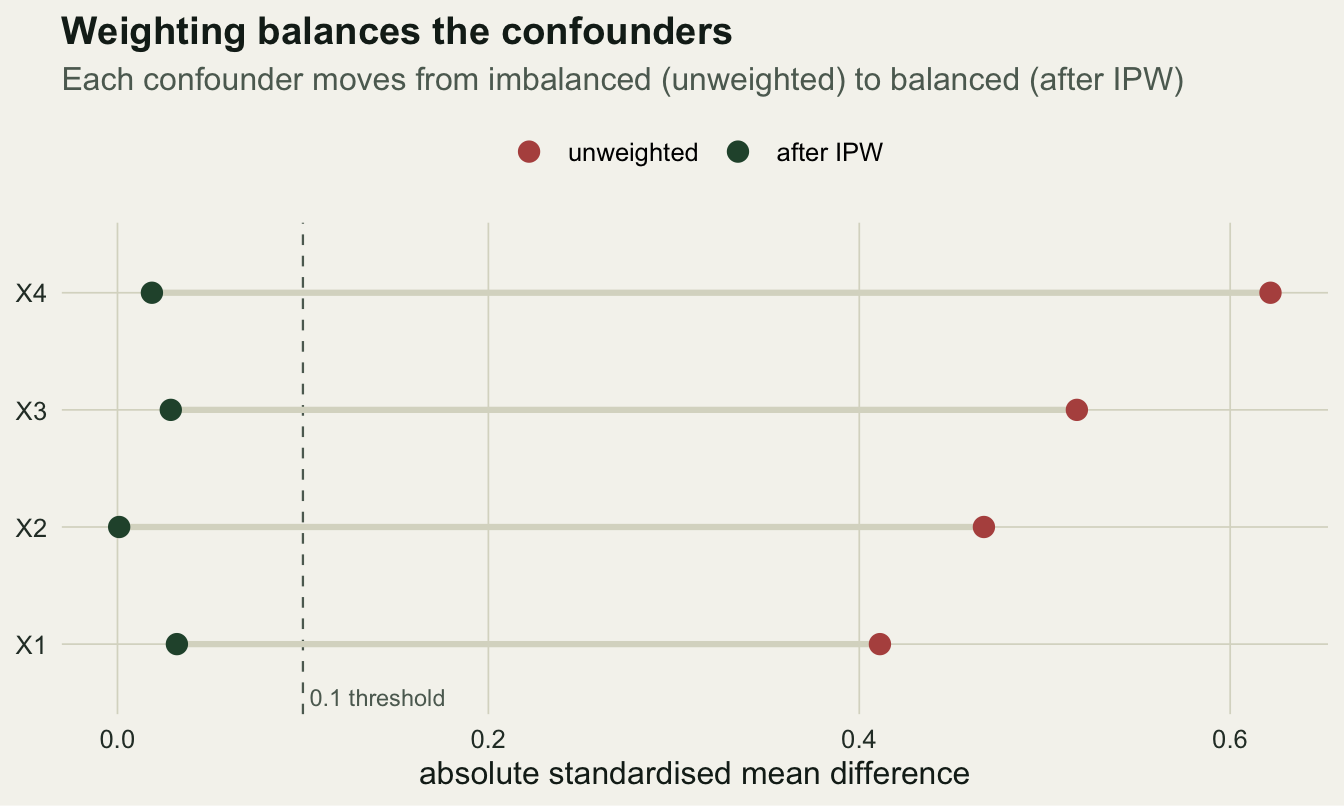
Overlap and positivity
Weighting only works where both groups exist. If some sites are almost certain to be treated (propensity near one) or almost certain not to be (near zero), their weights blow up and a handful of points dominate the estimate. The propensity distributions by group show whether there is common support.
e_range <- range(e); max_w <- max(w); ess <- sum(w)^2 / sum(w^2)Here the scores span 0.014 to 0.992, the largest weight is 19.6, and the effective sample size is 1281 of 2000: weighting spends about a third of the data buying balance. When a group thins out near zero or one, trimming extreme scores or switching to stabilised weights keeps a few points from taking over.
ov <- data.frame(e=e, grp=factor(ifelse(D==1,"treated","control"), levels=c("control","treated")))
ggplot(ov, aes(e, fill=grp, colour=grp)) +
  geom_density(alpha=0.35, linewidth=0.6) +
  scale_fill_manual(values=c("control"=brick,"treated"=forest), name=NULL) +
  scale_colour_manual(values=c("control"=brick,"treated"=forest), name=NULL) +
  labs(x="estimated propensity score  P(treated | confounders)", y="density",
       title="Overlap: both groups appear across the propensity range",
       subtitle="Mass near 0 and 1 produces large weights and strains positivity") +
  theme_te()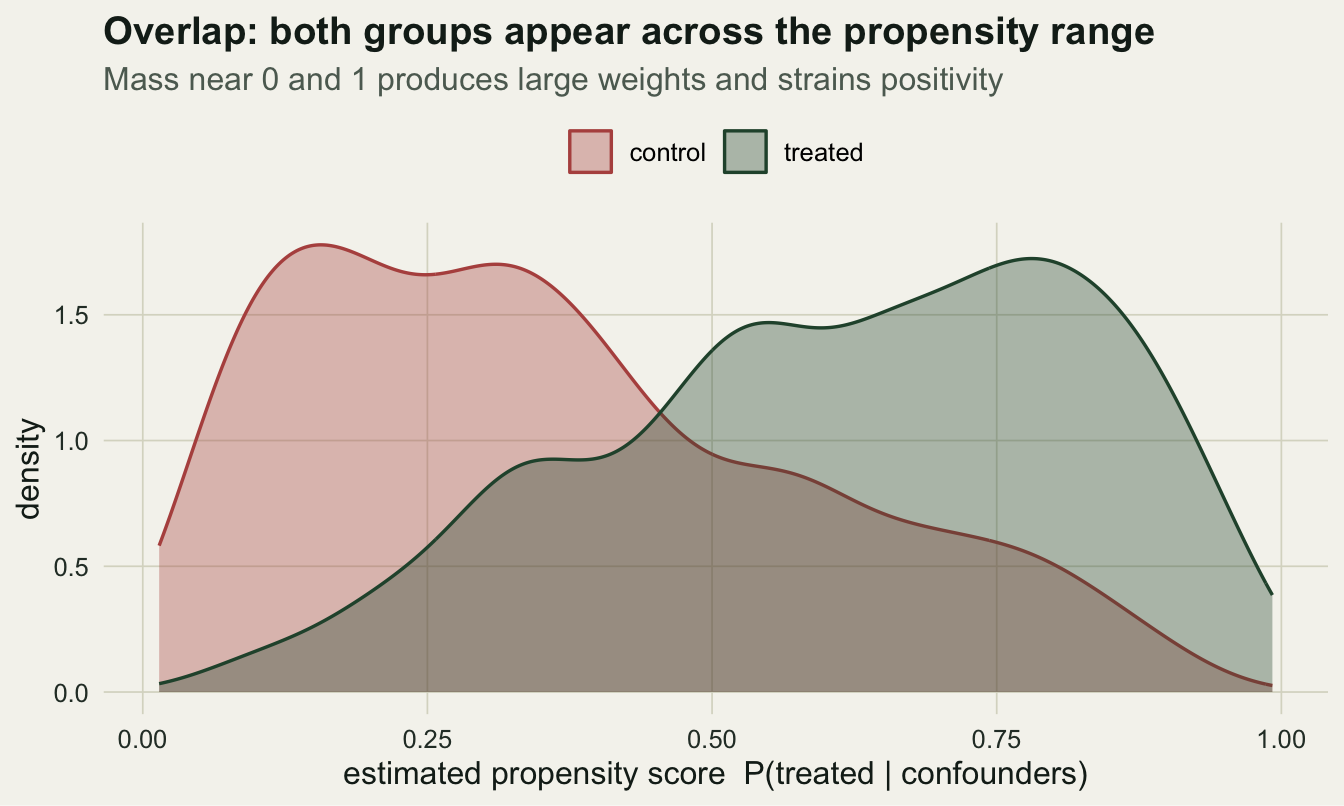
What breaks it: a missing confounder
Balance on the covariates in the model says nothing about a covariate left out. If a real confounder is missing from the propensity model, weighting cannot balance it, and the estimate stays biased. Drop the fourth covariate from the treatment model and the effect is wrong again.
ps_mis <- glm(D ~ X1+X2+X3, family=binomial)          # X4 omitted
w_mis  <- D/fitted(ps_mis) + (1-D)/(1-fitted(ps_mis))
ipw_mis <- coef(lm(Y ~ D, weights=w_mis))["D"]
With the fourth confounder left out, the estimate returns to 1.662, close to the naive value: no amount of weighting recovers what the model never saw. A short run across many datasets makes the contrast plain.
set.seed(9165); nsim <- 400
mc <- t(sapply(1:nsim, function(s){
  X1<-rnorm(n);X2<-rnorm(n);X3<-rnorm(n);X4<-rnorm(n)
  D <- rbinom(n,1, plogis(0.5*X1+0.7*X2-0.6*X3+0.8*X4))
  Y <- tau*D + 1.0*X1 + 0.8*X2 + 1.2*X3 + 0.9*X4 + rnorm(n,0,1)
  nv <- mean(Y[D==1]) - mean(Y[D==0])
  ee <- fitted(glm(D~X1+X2+X3+X4, family=binomial)); ww <- D/ee + (1-D)/(1-ee)
  c(naive=nv, ipw=unname(coef(lm(Y~D, weights=ww))["D"]))
}))
Averaged over 400 datasets the naive estimator sits at 1.781, the weighted estimator at 0.997: one systematically wrong, the other on target.
What the score buys, and what it assumes
Inverse-probability weighting turns a non-random treatment into a balanced comparison and recovers the effect, and unlike an outcome model it lets you audit that balance covariate by covariate before looking at the outcome. Three assumptions travel with it. No unmeasured confounding: every covariate that drives both treatment and outcome must be in the propensity model, which the balance check cannot vouch for. Positivity: both groups must appear across the covariate space, or the weights explode and rest on a few points. And a correctly specified propensity model, since a badly fitted score balances nothing. In ecology, where treatments are assigned by managers and geography rather than by chance, propensity methods are a natural fit and increasingly used (Ramsey et al. 2019; Butsic et al. 2017).
References
Rosenbaum PR, Rubin DB 1983. Biometrika 70(1):41-55 (10.1093/biomet/70.1.41).
Robins JM, Hernan MA, Brumback B 2000. Epidemiology 11(5):550-560 (10.1097/00001648-200009000-00011).
Austin PC 2011. Multivariate Behavioral Research 46(3):399-424 (10.1080/00273171.2011.568786).
Ramsey DSL, Forsyth DM, Wright E, McKay M, Westbrooke I 2019. Methods in Ecology and Evolution 10(3):320-331 (10.1111/2041-210X.13111).
Butsic V, Lewis DJ, Radeloff VC, Baumann M, Kuemmerle T 2017. Basic and Applied Ecology 19:1-10 (10.1016/j.baae.2017.01.005).
Larsen AE, Meng K, Kendall BE 2019. Methods in Ecology and Evolution 10(7):924-934 (10.1111/2041-210X.13190).