library(ggplot2); library(dplyr); library(tidyr)
paper<-"#f5f4ee"; ink<-"#16241d"; body<-"#2c3a31"; forest<-"#275139"
sage<-"#93a87f"; line<-"#dad9ca"; faint<-"#5d6b61"; brick<-"#b5534e"
theme_te <- function(base=12) theme_minimal(base_size=base) +
  theme(plot.background=element_rect(fill=paper,colour=NA),
        panel.background=element_rect(fill=paper,colour=NA),
        panel.grid.major=element_line(colour=line,linewidth=0.3),
        panel.grid.minor=element_blank(),
        axis.text=element_text(colour=body), axis.title=element_text(colour=ink),
        plot.title=element_text(colour=ink,face="bold"),
        plot.subtitle=element_text(colour=faint),
legend.position="top")Instrumental variables and 2SLS
R
causal inference
ecology tutorial
When an unmeasured confounder biases ordinary regression, a valid instrument and two-stage least squares can recover the causal effect. Built by hand in R.
Backdoor adjustment recovers a causal effect by conditioning on the confounders that open a spurious path (see confounding and backdoor adjustment). That recipe needs one thing we often lack: the confounder has to be measured. If soil productivity drives both grazing pressure and plant diversity but nobody recorded it, no regression of diversity on grazing can be trusted, and adding the covariates we happen to have does not fix the part we are missing.
An instrument offers a different route. Suppose some feature Z shifts the treatment X but has no path to the outcome Y except through X, and shares no common cause with Y. A topographic rule that sets stocking density, a distance that changes management access, a lottery that assigns a scheme: each nudges X while staying clear of the outcome’s confounders. The variation in Y that tracks Z can then be attributed to X, and the unmeasured confounding is stepped around rather than adjusted away. This tutorial builds the estimator by hand, shows when it works, and shows the two ways it fails.
A confounded example
We simulate a treatment X and outcome Y that share an unobserved confounder U. An instrument Z pushes X (strength a1) and is independent of U. The true effect of X on Y is 0.5.
set.seed(4163)
n <- 800; b_true <- 0.5; a1 <- 0.8
U <- rnorm(n)                          # unobserved confounder
Z <- rnorm(n)                          # instrument, independent of U
X <- 0.2 + a1*Z + 0.9*U + rnorm(n, 0, 0.7)
Y <- 1.0 + b_true*X + 0.8*U + rnorm(n, 0, 0.7)
Because U raises both X and Y, an ordinary regression of Y on X counts the confounding as if it were effect:
ols   <- lm(Y ~ X)
b_ols <- coef(ols)["X"]
ci_ols<- confint(ols)["X", ]
The naive slope is 0.882 with a 95% interval of [0.835, 0.93], far above the true 0.5 and confident about it. The interval never touches the truth: the bias is systematic, not sampling noise.
Two-stage least squares
The instrument isolates the part of X that has nothing to do with U. Regress X on Z and keep the fitted values (the first stage); then regress Y on those fitted values (the second stage). The slope of the second stage is the two-stage least squares (2SLS) estimate.
s1    <- lm(X ~ Z); Xhat <- fitted(s1)   # first stage
s2    <- lm(Y ~ Xhat)                     # second stage
b_2sls<- coef(s2)["Xhat"]
With one instrument this equals the ratio (Wald) estimator, the covariance of Y with Z divided by the covariance of X with Z:
b_wald <- cov(Y, Z) / cov(X, Z)
gap    <- b_2sls - b_wald
The two agree to within floating-point rounding. The estimate is 0.534, close to the true 0.5: the instrument recovered the effect that the confounder hid. The intuition is simple. Z moves X but not U, so the slice of Y that co-varies with Z can only have arrived through X.
Get the standard error from the structural equation
There is a trap in reading the second-stage regression’s reported error. That regression uses residuals of Y against the fitted Xhat, which are on the wrong scale; the correct variance uses residuals of the structural equation, Y minus the fitted line evaluated at the observed X.
uhat  <- Y - (coef(s2)[1] + b_2sls*X)     # structural residual
sig2  <- sum(uhat^2)/(n-2)
Xd    <- cbind(1, Xhat)
se_2sls<- sqrt((sig2 * solve(crossprod(Xd)))[2,2])
se_naive<- summary(s2)$coef["Xhat","Std. Error"]
ci_2sls<- b_2sls + c(-1,1)*qnorm(0.975)*se_2sls
The correct error is 0.048; the second stage’s own figure (0.066) misstates it, here overstating uncertainty because its residuals are taken against Xhat, so on top of the structural error they still carry the slope times the part of X the instrument discarded. The proper 95% interval is [0.44, 0.627], which contains 0.5.
est <- data.frame(
  method = factor(c("OLS (naive)","2SLS (instrument)"),
                  levels=c("OLS (naive)","2SLS (instrument)")),
  est = c(b_ols,b_2sls), lo = c(ci_ols[1],ci_2sls[1]), hi = c(ci_ols[2],ci_2sls[2]))
ggplot(est, aes(method, est, colour=method)) +
  geom_hline(yintercept=b_true, linetype="dashed", colour=ink, linewidth=0.5) +
  geom_errorbar(aes(ymin=lo, ymax=hi), width=0.12, linewidth=0.8) +
  geom_point(size=3.4) +
  scale_colour_manual(values=c("OLS (naive)"=brick,"2SLS (instrument)"=forest), guide="none") +
  labs(x=NULL, y="estimated effect of X on Y",
       title="Instrument recovers the effect an unmeasured confounder hides",
       subtitle="Dashed line: true effect (0.5). Naive OLS is biased upward; 2SLS straddles the truth") +
  theme_te()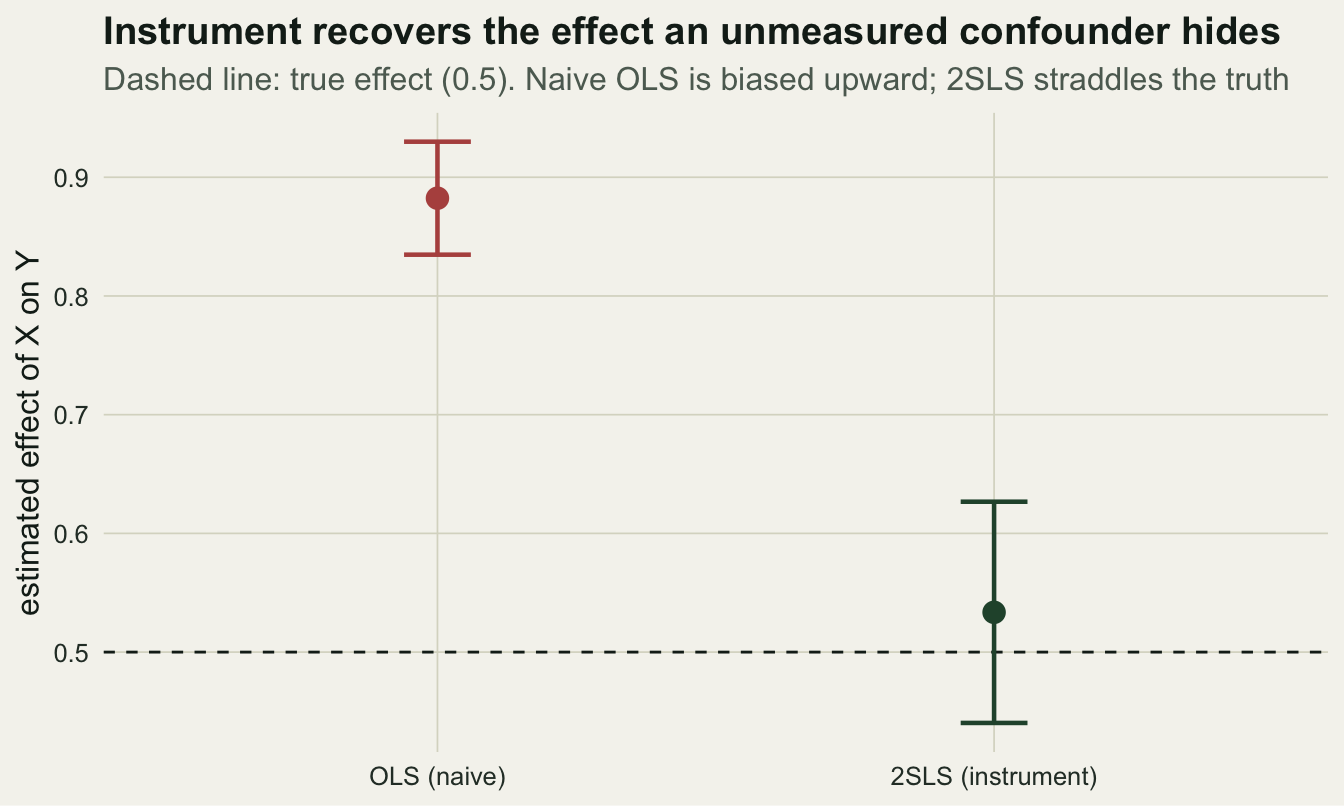
Instrument strength and the weak-instrument trap
The Wald estimator divides by the covariance of X with Z. When the instrument is weak that denominator is near zero, and dividing by a small, noisy number gives a wild, biased estimate. The first-stage F statistic measures strength; with a single instrument it is the square of the first-stage t.
a1_hat <- coef(s1)["Z"]
Fstat  <- summary(s1)$coef["Z","t value"]^2
r2s1   <- summary(s1)$r.squared
Here the first stage is strong: the coefficient on Z is 0.797, the F statistic is 389, and Z explains 33% of the variation in X. A sweep across instrument strengths shows what happens as the first stage weakens.
strengths <- c(0.05,0.1,0.2,0.4,0.8); nsim <- 1000
set.seed(50)
sweep <- lapply(strengths, function(a){
  bb <- Fv <- numeric(nsim)
  for (i in 1:nsim){
    U <- rnorm(n); Z <- rnorm(n)
    X <- 0.2 + a*Z + 0.9*U + rnorm(n,0,0.7)
    Y <- 1.0 + b_true*X + 0.8*U + rnorm(n,0,0.7)
    bb[i] <- cov(Y,Z)/cov(X,Z)
    Fv[i] <- summary(lm(X~Z))$coef["Z","t value"]^2
  }
  q <- quantile(bb, c(.25,.5,.75))
  data.frame(strength=a, medF=median(Fv), p25=q[1], med=q[2], p75=q[3], sdEst=sd(bb))
}) %>% bind_rows()
At a strong first stage (F near 395) the median estimate is 0.5 with a standard deviation of 0.049. At a weak first stage (F near 1.6) the median drifts up to 0.63, back toward the confounded OLS slope, and the spread explodes (standard deviation 25.6). The rule of thumb from Staiger and Stock is a first-stage F above about 10; below it, inference cannot be believed.
ggplot(sweep, aes(medF, med)) +
  geom_ribbon(aes(ymin=p25, ymax=p75), fill=sage, alpha=0.35) +
  geom_hline(yintercept=b_true, linetype="dashed", colour=forest, linewidth=0.5) +
  geom_hline(yintercept=b_ols, linetype="dotted", colour=brick, linewidth=0.5) +
  geom_vline(xintercept=10, linetype="dashed", colour=faint, linewidth=0.4) +
  geom_line(colour=ink, linewidth=0.6) + geom_point(colour=forest, size=2.6) +
  annotate("text", x=10, y=1.35, label="F = 10", hjust=-0.1, colour=faint, size=3.2) +
  annotate("text", x=1.5, y=b_ols+0.05, label="OLS limit", hjust=0, colour=brick, size=3.2) +
  annotate("text", x=200, y=b_true-0.09, label="truth", hjust=1, colour=forest, size=3.2) +
  scale_x_log10() + coord_cartesian(ylim=c(-0.2,1.4)) +
  labs(x="first-stage F statistic (log scale)", y="2SLS estimate (median, 25-75%)",
       title="Weak instruments bias 2SLS toward OLS and inflate its variance",
       subtitle="As the instrument weakens, the estimate drifts toward the confounded slope") +
  theme_te()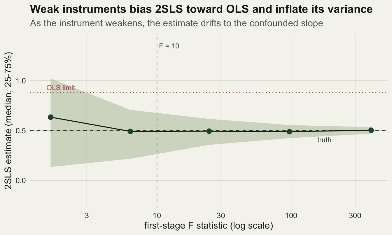
What can break it: the exclusion restriction
The estimator leans on an assumption the data cannot check: Z affects Y only through X. If Z has any direct path to Y, however small, 2SLS is biased, and the bias is the direct effect divided by the instrument strength. A weak instrument magnifies even a tiny leak.
set.seed(9163); gamma <- 0.15
excl <- lapply(c(0.8,0.2), function(a){
  bb <- numeric(600)
  for (i in 1:600){
    U <- rnorm(n); Z <- rnorm(n)
    X <- 0.2 + a*Z + 0.9*U + rnorm(n,0,0.7)
    Y <- 1.0 + b_true*X + 0.8*U + gamma*Z + rnorm(n,0,0.7)   # direct Z to Y
    bb[i] <- cov(Y,Z)/cov(X,Z)
  }
  data.frame(strength=a, bias=mean(bb)-b_true, approx=gamma/a)
}) %>% bind_rows()
With a direct effect of 0.15 planted from Z to Y, a strong instrument (strength 0.8) shows a bias of 0.186, matching the predicted 0.187. A weak instrument (strength 0.2) turns the same leak into a bias of 0.748, near the predicted 0.75. The exclusion restriction is a judgement about the system, argued from how the instrument works, never confirmed from the numbers.
What the instrument buys
A closing check compares interval coverage across many datasets: does the 95% interval contain the truth 95% of the time?
set.seed(7163); ncov <- 1200; cov_ols <- cov_iv <- logical(ncov)
for (i in 1:ncov){
  U <- rnorm(n); Z <- rnorm(n)
  X <- 0.2 + 0.8*Z + 0.9*U + rnorm(n,0,0.7)
  Y <- 1.0 + b_true*X + 0.8*U + rnorm(n,0,0.7)
  o <- lm(Y~X); ci <- confint(o)["X",]; cov_ols[i] <- b_true>=ci[1] & b_true<=ci[2]
  Xh <- fitted(lm(X~Z)); s <- lm(Y~Xh); bh <- coef(s)[2]
  uh <- Y-(coef(s)[1]+bh*X); v <- sum(uh^2)/(n-2)
  se <- sqrt((v*solve(crossprod(cbind(1,Xh))))[2,2])
  cih <- bh+c(-1,1)*qnorm(0.975)*se; cov_iv[i] <- b_true>=cih[1] & b_true<=cih[2]
}
The ordinary interval covers the truth 0% of the time: it is precise and wrong. The 2SLS interval covers 95.2%, close to nominal. That gain is not free. It rests on a strong first stage, on independence of Z from the confounders, and on the exclusion restriction, and none of these follow from a good model fit. When an instrument is available and defensible, it reaches an effect that adjustment cannot; when it is weak or leaky, it can be worse than the naive slope it was meant to repair. In ecology the honest move is to state the assumed causal structure and treat the instrument as a design choice, not a computation (Butsic et al. 2017; Larsen, Meng & Kendall 2019).
References
Angrist JD, Imbens GW, Rubin DB 1996. Journal of the American Statistical Association 91(434):444-455 (10.1080/01621459.1996.10476902).
Bound J, Jaeger DA, Baker RM 1995. Journal of the American Statistical Association 90(430):443-450 (10.1080/01621459.1995.10476536).
Staiger D, Stock JH 1997. Econometrica 65(3):557-586 (10.2307/2171753).
Butsic V, Lewis DJ, Radeloff VC, Baumann M, Kuemmerle T 2017. Basic and Applied Ecology 19:1-10 (10.1016/j.baae.2017.01.005).
Larsen AE, Meng K, Kendall BE 2019. Methods in Ecology and Evolution 10(7):924-934 (10.1111/2041-210X.13190).
Arif S, MacNeil MA 2022. Ecosphere 13(4):e4009 (10.1002/ecs2.4009).