library(ggplot2)

te_pal <- list(forest = "#275139", green = "#2f8f63", sage = "#93a87f",
               clay = "#b5534e", gold = "#cda23f", line = "#dad9ca",
               ink = "#16241d", paper = "#f5f4ee")

theme_te <- function() {
  theme_minimal(base_size = 12) +
    theme(panel.grid.minor = element_blank(),
          panel.grid.major = element_line(colour = "#e7e6dc"),
          plot.background = element_rect(fill = "#f5f4ee", colour = NA),
          panel.background = element_rect(fill = "#f5f4ee", colour = NA),
          plot.title = element_text(face = "bold", colour = te_pal$ink),
          axis.title = element_text(colour = "#2c3a31"),
          axis.text = element_text(colour = "#2c3a31"))
}Baseline selection and the return to the mean
R
experimental design
causal inference
monitoring
ecology tutorial
Targeting the worst sites manufactures a treatment effect. How large it gets, why parallel-trends diagnostics never fire, and which baseline design removes it.
A catchment programme has money for eighty stream reaches. The monitoring network covers four hundred of them, each kick-sampled once a year and scored on a macroinvertebrate condition index, and six years of scores are already in the database. Choosing where the money goes takes one line of code: sort by the six-year mean and take the bottom fifth. Those are the reaches in trouble, and they get the fencing, the woody debris and the buffer planting. Five years later the programme is evaluated with a difference-in-differences contrast against the reaches that were not treated, and it reports a gain, with a confidence interval that excludes zero.
In the simulation below the treatment effect is exactly zero. Nothing was done to any reach. The gain is manufactured by the selection rule, and the mechanism is old: a reach that scored badly in the baseline window scored badly partly because its true condition is poor and partly because it had a bad run of years, and the bad run does not repeat. The luck component reverts, the true component stays, and the reverting part is read as recovery. Barnett, van der Pols and Dobson (2005) give the general account of that arithmetic and of what to do about it; Kelly and Price (2005) work the same problem for behaviour and ecology, where the repeated measurement is a trait score rather than a blood pressure.
That much is standard textbook material. The part that is not standard, and the reason this post exists next to the ones below, is what the usual defences do about it. Before-after-control-impact designs already builds a confident spurious impact and says so plainly: there, “the disturbance does nothing; the impact site simply drifts downward on its own”, and the interaction “excluding zero: a confident, entirely spurious impact, manufactured by a background trend the control did not share”. Its prescription is more before periods, so that you can see whether the trends really run parallel, and event-study difference-in-differences turns those pre-intervention periods into “a visible diagnostic”. Mean reversion is not a differential trend. The leads sit on zero, the placebo in time is null, the estimate is still wrong, and no amount of extra data makes the diagnostic fire.
Three neighbouring posts deal with adjacent problems and not with this one. Restoration trajectories and recovery has selection running the other way, towards the sites that were easiest and best, so that site age and site quality end up correlated in a chronosequence. Checking an Allee analysis uses regression to the mean in its within-series form, where the same noisy count sets the x axis and the y axis of one scatter and manufactures density dependence; here the noise is shared between a selection rule and a baseline value rather than between two axes. Checking a monitoring design loses sites to dropout, which changes who is measured rather than who is treated.
Five measurements follow: how big the manufactured effect is and what it depends on, what the standard pre-trend diagnostics report while it happens, what three ordinary analyses of the same table say about it, why they disagree, and which changes to the baseline design remove it.
A programme that targets the worst reaches
Each reach has a true condition that does not change over the study, and each annual visit adds an independent departure from it: a spate that scoured the riffle, a warm summer, a sampler who worked the margins rather than the centre. Treatment goes to the reaches with the lowest six-year mean, but not purely: which of the poor reaches can actually be worked depends on access and on whether the landowner agrees, so an administrative term enters the ranking alongside the monitoring score. That term matters later, because without it treatment would be a deterministic function of the baseline and one of the three analyses below would not be estimable at all.
n_site   <- 400
n_pre    <- 6
n_post   <- 5
sd_site  <- 10
sd_year  <- 14
mu_base  <- 48
sd_admin <- 8
k_frac   <- 0.20

make_panel <- function(seed, sd_yr = sd_year, ns = n_site, npre = n_pre,
                       npost = n_post, frac = k_frac, drift = 0,
                       rule = "baseline") {
  set.seed(seed)
  quality <- rnorm(ns, mu_base, sd_site)
  n_yr <- npre + npost
  obs <- quality + matrix(rnorm(ns * n_yr, 0, sd_yr), ns, n_yr)
  admin <- rnorm(ns, 0, sd_admin)
  score <- switch(rule,
                  baseline = rowMeans(obs[, seq_len(npre), drop = FALSE]) + admin,
                  quality  = quality + admin,
                  random   = admin)
  treated <- rep(0L, ns)
  treated[order(score)[seq_len(round(ns * frac))]] <- 1L
  if (drift != 0) obs <- obs + drift * (treated %o% (seq_len(n_yr) - (npre + 1)))
  list(obs = obs, quality = quality, treated = treated,
       npre = npre, npost = npost)
}

pre_mean  <- function(p) rowMeans(p$obs[, seq_len(p$npre), drop = FALSE])
post_mean <- function(p) rowMeans(p$obs[, p$npre + seq_len(p$npost), drop = FALSE])

rel_one <- sd_site^2 / (sd_site^2 + sd_year^2)
rel_pre <- sd_site^2 / (sd_site^2 + sd_year^2 / n_pre)
lam_pre <- 1 - rel_pre

print(c(reaches = n_site, treated = n_site * k_frac, pre_years = n_pre,
        post_years = n_post, true_effect = 0))
reaches treated pre_years post_years true_effect
400 80 6 5 0 print(round(c(site_sd = sd_site, year_sd = sd_year,
reliability_one_year = rel_one,
reliability_six_year_mean = rel_pre,
noise_share_of_baseline = lam_pre), 4)) site_sd year_sd reliability_one_year
10.0000 14.0000 0.3378
reliability_six_year_mean noise_share_of_baseline
0.7538 0.2462 A single year’s index at a reach has a reliability of 0.3378: two thirds of the spread across reaches in any one year is the year rather than the reach. Averaging six years raises that to 0.7538, so the baseline value used for selection is mostly signal. The leftover noise share, 0.2462, is the quantity that does all the damage below.
prog <- make_panel(20260801)
base_val <- pre_mean(prog)
post_val <- post_mean(prog)
tw <- prog$treated
chg <- post_val - base_val

fit_did <- lm(chg ~ tw)
did_est <- unname(coef(fit_did)[2])
did_ci <- confint(fit_did)[2, ]
did_p <- summary(fit_did)$coefficients[2, 4]
gap_obs <- mean(base_val[tw == 0]) - mean(base_val[tw == 1])
gap_true <- mean(prog$quality[tw == 0]) - mean(prog$quality[tw == 1])

print(round(summary(fit_did)$coefficients, 5))
Estimate Std. Error t value Pr(>|t|)
(Intercept) 0.61621 0.46313 1.33053 0.18410
tw 2.76240 1.03558 2.66749 0.00795print(round(c(did = did_est, lower = did_ci[1], upper = did_ci[2], p = did_p,
observed_baseline_gap = gap_obs, true_condition_gap = gap_true,
predicted_bias = lam_pre * gap_obs), 4)) did lower.2.5 % upper.97.5 %
2.7624 0.7265 4.7983
p observed_baseline_gap true_condition_gap
0.0080 17.5841 13.7039
predicted_bias
4.3297 The programme reports a gain of 2.762 index points, interval 0.727 to 4.798, p of 0.00795, against a true effect of zero. The treated reaches did start 17.584 points below the others on the observed baseline, and 13.704 points below on their true condition. The gap in observed baseline is larger than the gap in truth, and the difference between the two is the whole story: 3.88 points of the apparent baseline deficit was never there.
The manufactured effect has a formula
The size of the artefact is not something to guess at. Write the baseline value as true condition plus a baseline noise term, and the selection score as that same baseline value plus the administrative term. The change score removes the true condition, because it is the same before and after, so the whole difference-in-differences estimate is the difference in baseline noise between the arms, with the sign flipped. Projecting the noise onto the selection score gives an expected estimate of the noise share of the baseline multiplied by the observed baseline gap. Both of those are things you can compute from your own data before the follow-up is collected.
n_rep_a <- 400
rep_did <- rep_gap <- numeric(n_rep_a)
for (r in seq_len(n_rep_a)) {
  p <- make_panel(50000 + r)
  bb <- pre_mean(p); pp <- post_mean(p); zz <- p$treated
  rep_did[r] <- mean((pp - bb)[zz == 1]) - mean((pp - bb)[zz == 0])
  rep_gap[r] <- mean(bb[zz == 0]) - mean(bb[zz == 1])
}
did_mean <- mean(rep_did)
did_mcse <- sd(rep_did) / sqrt(n_rep_a)
gap_mean <- mean(rep_gap)
ratio_meas <- did_mean / gap_mean

print(round(c(replicates = n_rep_a, mean_did = did_mean, mc_se = did_mcse,
              mean_baseline_gap = gap_mean, measured_ratio = ratio_meas,
              predicted_ratio = lam_pre,
              predicted_did = lam_pre * gap_mean), 5))
replicates mean_did mc_se mean_baseline_gap
400.00000 4.03037 0.05167 16.54999
measured_ratio predicted_ratio predicted_did
0.24353 0.24623 4.07512 Over 400 replicate programmes the average manufactured effect is 4.0304 points with a Monte Carlo standard error of 0.0517, and the ratio of that to the average observed baseline gap is 0.24353 against a predicted 0.24623. In index points the prediction is 4.0751 points, which sits 0.0447 above the measured mean and inside one Monte Carlo standard error of it.
The next question is what the ratio depends on. Two candidates present themselves: how noisy the index is, and how hard the programme targets. Only one of them matters much.
nsr_grid <- seq_len(8) / 10
frac_grid <- c(0.05, 0.20, 0.50)
n_rep_s <- 150
sw_rows <- list()
for (nsr in nsr_grid) for (fr in frac_grid) {
  sdy <- sd_site * sqrt(nsr / (1 - nsr))
  dv <- gv <- numeric(n_rep_s)
  for (r in seq_len(n_rep_s)) {
    p <- make_panel(90000 + r, sd_yr = sdy, frac = fr)
    bb <- pre_mean(p); pp <- post_mean(p); zz <- p$treated
    dv[r] <- mean((pp - bb)[zz == 1]) - mean((pp - bb)[zz == 0])
    gv[r] <- mean(bb[zz == 0]) - mean(bb[zz == 1])
  }
  sw_rows[[length(sw_rows) + 1]] <- data.frame(
    noise_share = nsr, frac = fr, did = mean(dv), gap = mean(gv),
    ratio = mean(dv) / mean(gv),
    lambda = (sdy^2 / n_pre) / (sd_site^2 + sdy^2 / n_pre))
}
sw1 <- do.call(rbind, sw_rows)
print(round(sw1, 4))
noise_share frac did gap ratio lambda
1 0.1 0.05 0.3398 17.0958 0.0199 0.0182
2 0.1 0.20 0.2410 13.7725 0.0175 0.0182
3 0.1 0.50 0.2362 12.6248 0.0187 0.0182
4 0.2 0.05 0.7503 17.3890 0.0431 0.0400
5 0.2 0.20 0.5431 13.9509 0.0389 0.0400
6 0.2 0.50 0.5282 12.8124 0.0412 0.0400
7 0.3 0.05 1.2434 17.7259 0.0701 0.0667
8 0.3 0.20 0.9227 14.2298 0.0648 0.0667
9 0.3 0.50 0.8903 13.0721 0.0681 0.0667
10 0.4 0.05 1.8409 18.1477 0.1014 0.1000
11 0.4 0.20 1.4360 14.5866 0.0984 0.1000
12 0.4 0.50 1.3675 13.4040 0.1020 0.1000
13 0.5 0.05 2.6501 18.6802 0.1419 0.1429
14 0.5 0.20 2.0876 15.0417 0.1388 0.1429
15 0.5 0.50 2.0237 13.8319 0.1463 0.1429
16 0.6 0.05 3.9426 19.5157 0.2020 0.2000
17 0.6 0.20 3.1038 15.7579 0.1970 0.2000
18 0.6 0.50 2.9513 14.4720 0.2039 0.2000
19 0.7 0.05 5.9241 20.9240 0.2831 0.2800
20 0.7 0.20 4.7259 16.8581 0.2803 0.2800
21 0.7 0.50 4.4463 15.5430 0.2861 0.2800
22 0.8 0.05 9.3216 23.5058 0.3966 0.4000
23 0.8 0.20 7.6733 19.0219 0.4034 0.4000
24 0.8 0.50 7.0787 17.4655 0.4053 0.4000pick <- function(nsr, fr, col) {
i <- which(abs(sw1$noise_share - nsr) < 1e-8 & abs(sw1$frac - fr) < 1e-8)
stopifnot(length(i) == 1)
sw1[[col]][i]
}
print(round(c(noise_effect_at_worst20 = pick(0.7, 0.2, "did") /
pick(0.2, 0.2, "did"),
intensity_effect_at_ns07 = pick(0.7, 0.05, "did") /
pick(0.7, 0.5, "did"),
max_ratio_spread_across_intensities =
max(tapply(sw1$ratio, sw1$noise_share,
function(v) max(v) - min(v)))), 4)) noise_effect_at_worst20 intensity_effect_at_ns07
8.7009 1.3324
max_ratio_spread_across_intensities
0.0087 ratio_spread <- max(tapply(sw1$ratio, sw1$noise_share,
function(v) max(v) - min(v)))Holding the targeting fixed at the worst fifth and moving the noise share of a single year’s index from 0.2 to 0.7 multiplies the manufactured effect by 8.701. Holding the noise at 0.7 and going from the worst half to the worst twentieth multiplies it by only 1.332. This is not what I expected before running the sweep. Aggressive targeting feels like the reckless part of the design, and it is close to irrelevant: it widens the observed baseline gap a little, and the fraction of that gap which reverts does not depend on it at all. At every noise level the three selection intensities give ratios lying within 0.0087 of each other, and all of them track the predicted noise share of the baseline mean.
lab_int <- c("worst 5 per cent", "worst 20 per cent", "worst 50 per cent")
sw1$intensity <- factor(lab_int[match(sw1$frac, frac_grid)], levels = lab_int)
pan <- c("Manufactured effect (index points)",
         "Effect as a share of the observed baseline gap")
fig1 <- rbind(
  data.frame(noise_share = sw1$noise_share, intensity = sw1$intensity,
             value = sw1$did, panel = pan[1]),
  data.frame(noise_share = sw1$noise_share, intensity = sw1$intensity,
             value = sw1$ratio, panel = pan[2]))
fig1$panel <- factor(fig1$panel, levels = pan)

ggplot(fig1, aes(noise_share, value, colour = intensity, shape = intensity)) +
  geom_line(linewidth = 0.7) +
  geom_point(size = 2.1) +
  facet_wrap(~panel, scales = "free_y") +
  scale_colour_manual(values = c(te_pal$clay, te_pal$forest, te_pal$gold),
                      name = NULL) +
  scale_shape_manual(values = c(16, 17, 15), name = NULL) +
  labs(x = "noise share of a single year's index",
       y = NULL,
       title = "Noise decides the size; targeting barely does") +
  theme_te() +
  theme(legend.position = "bottom", plot.margin = margin(8, 14, 4, 8))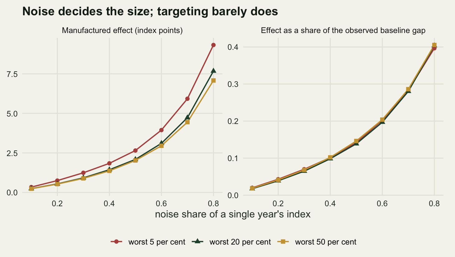
The diagnostics that do not fire
The recommended defence against a spurious impact is to look at the pre-intervention periods. Fit a coefficient for each year relative to the last pre-intervention year, check that the ones before the intervention sit on zero, and run the treatment date backwards into the pre-period to see whether the design produces an effect where there cannot be one. Larsen, Meng and Kendall (2019) bring that econometric apparatus across to ecological control-impact studies and set out what each check does and does not establish. Both checks are run below on two datasets: the mean-reversion programme, and a second one in which treatment is allocated at random and the treated reaches carry a linear differential trend. The trend is calibrated so the two datasets return the same difference-in-differences estimate. They differ only in how it was manufactured.
lever <- mean(seq_len(n_post) - 1) - mean(-n_pre:-1)
drift_cal <- did_mean / lever
p_mr <- make_panel(410001)
p_dt <- make_panel(420001, rule = "random", drift = drift_cal)

ev_gaps <- function(p) {
  g <- colMeans(p$obs[p$treated == 1, , drop = FALSE]) -
       colMeans(p$obs[p$treated == 0, , drop = FALSE])
  unname(g - g[p$npre])
}

es_fit <- function(p) {
  ns <- nrow(p$obs); n_yr <- ncol(p$obs)
  dat <- data.frame(y = as.vector(p$obs),
                    id = factor(rep(seq_len(ns), n_yr)),
                    yr = factor(rep(seq_len(n_yr), each = ns)),
                    zz = rep(p$treated, n_yr),
                    ev = rep(seq_len(n_yr) - (p$npre + 1), each = ns))
  kv <- setdiff(sort(unique(dat$ev)), -1)
  X <- sapply(kv, function(kk) as.integer(dat$zz == 1 & dat$ev == kk))
  colnames(X) <- paste0("k", ifelse(kv < 0, paste0("m", abs(kv)), kv))
  m <- lm(as.formula(paste("y ~ id + yr +", paste(colnames(X), collapse = "+"))),
          cbind(dat, as.data.frame(X)))
  co <- summary(m)$coefficients[colnames(X), 1:2]
  data.frame(k = kv, est = co[, 1], se = co[, 2], row.names = NULL)
}

es_mr <- es_fit(p_mr)
es_dt <- es_fit(p_dt)
check_mr <- max(abs(es_mr$est - ev_gaps(p_mr)[-n_pre]))
print(round(cbind(es_mr, dt_est = es_dt$est, dt_se = es_dt$se), 4))
k est se dt_est dt_se
1 -6 -0.8114 2.4026 -5.9278 2.4481
2 -5 0.5973 2.4026 -3.9603 2.4481
3 -4 1.6433 2.4026 -2.5024 2.4481
4 -3 -0.5263 2.4026 -0.9540 2.4481
5 -2 -2.5799 2.4026 0.1283 2.4481
6 0 3.6875 2.4026 1.3484 2.4481
7 1 2.0699 2.4026 0.0144 2.4481
8 2 0.6399 2.4026 1.4522 2.4481
9 3 0.4307 2.4026 1.4626 2.4481
10 4 2.7819 2.4026 1.5838 2.4481print(round(c(calibrated_drift = drift_cal, event_time_lever = lever,
closed_form_vs_lm = check_mr), 6)) calibrated_drift event_time_lever closed_form_vs_lm
0.732795 5.500000 0.000000 The estimator is the standard two-way fixed-effects event study: reach effects, year effects, and one indicator per event time for the treated group, with the year before the intervention left out. In a balanced two-group panel its coefficients are exactly the treated-minus-control gap in each year minus that gap in the reference year, which is what the last printed line confirms to machine precision. One realisation of each dataset is noisy, so the same paths are averaged over replicates below.
n_rep_e <- 300
path_mr <- t(sapply(seq_len(n_rep_e),
                    function(i) ev_gaps(make_panel(50000 + i))))
path_dt <- t(sapply(seq_len(n_rep_e),
                    function(i) ev_gaps(make_panel(60000 + i, rule = "random",
                                                   drift = drift_cal))))
ev_time <- seq_len(n_pre + n_post) - (n_pre + 1)
lead_idx <- which(ev_time < -1)
mr_leads <- colMeans(path_mr)[lead_idx]
dt_leads <- colMeans(path_dt)[lead_idx]
mr_lag <- mean(colMeans(path_mr)[ev_time >= 0])
dt_lag <- mean(colMeans(path_dt)[ev_time >= 0])
path_mcse <- apply(path_mr, 2, sd) / sqrt(n_rep_e)
did_of <- function(m) mean(rowMeans(m[, ev_time >= 0]) -
                             rowMeans(m[, ev_time < 0]))

print(round(rbind(event_time = ev_time,
                  mean_reversion = colMeans(path_mr),
                  differential_trend = colMeans(path_dt),
                  mc_se = path_mcse), 4))
[,1] [,2] [,3] [,4] [,5] [,6] [,7] [,8]
event_time -6.0000 -5.0000 -4.0000 -3.0000 -2.0000 -1 0.0000 1.0000
mean_reversion -0.1604 -0.0190 -0.0730 -0.1241 -0.1009 0 4.0652 3.9267
differential_trend -3.5504 -2.7845 -2.2890 -1.4173 -0.5197 0 0.8895 1.6018
mc_se 0.1486 0.1519 0.1572 0.1411 0.1578 0 0.1480 0.1502
[,9] [,10] [,11]
event_time 2.0000 3.0000 4.0000
mean_reversion 3.8926 3.8570 4.0588
differential_trend 2.1406 3.0724 3.8636
mc_se 0.1451 0.1466 0.1452print(round(c(max_abs_lead_mean_reversion = max(abs(mr_leads)),
max_mc_se_over_leads = max(path_mcse[lead_idx]),
lead_span_differential_trend = max(dt_leads) - min(dt_leads),
mean_lag_mean_reversion = mr_lag,
mean_lag_differential_trend = dt_lag,
did_mean_reversion = did_of(path_mr),
did_differential_trend = did_of(path_dt)), 4)) max_abs_lead_mean_reversion max_mc_se_over_leads
0.1604 0.1578
lead_span_differential_trend mean_lag_mean_reversion
3.0307 3.9600
mean_lag_differential_trend did_mean_reversion
2.3136 4.0396
did_differential_trend
4.0737 The five estimable lead coefficients under mean reversion have a largest absolute value of 0.1604 index points, against a Monte Carlo standard error of 0.1578 on each. They are zero, and they are zero for a reason rather than by luck: selection was on the mean of the six pre-intervention years, so every one of those years carries the same share of the selection noise and the treated-minus-control gap is identical in all of them. That flatness is a property of the selection rule and not of mean reversion. When the rule reads a single period instead, the reverting component does show up in the leads, which is what Ashenfelter (1978) found in the earnings of training participants: a dip in the year before enrolment, visible precisely because enrolment followed that one year. The post-intervention coefficients average 3.96 and are flat, which reads as an effect that arrived immediately and held.
Under the differential trend the same code returns leads spanning 3.0307 points and marching in one direction, with post-intervention coefficients that ramp rather than step, averaging 2.3136. The two datasets are calibrated to agree on the thing that gets reported: the difference-in-differences contrast is 4.0396 in the first and 4.0737 in the second. One of these two figures has a diagnostic in it. The other does not.
pan_dgp <- c("Mean reversion: selection on the baseline",
             "Differential trend: random selection")
band <- function(m, nm) data.frame(
  k = ev_time, mid = colMeans(m),
  lo = apply(m, 2, quantile, 0.05), hi = apply(m, 2, quantile, 0.95),
  dgp = nm)
fig2 <- rbind(band(path_mr, pan_dgp[1]), band(path_dt, pan_dgp[2]))
fig2$dgp <- factor(fig2$dgp, levels = pan_dgp)
fig2$side <- ifelse(fig2$k < 0, "pre", "post")

ggplot(fig2, aes(k, mid)) +
  geom_hline(yintercept = 0, colour = te_pal$line, linewidth = 0.5) +
  geom_vline(xintercept = -0.5, linetype = "dashed",
             colour = te_pal$ink, linewidth = 0.5) +
  geom_ribbon(aes(ymin = lo, ymax = hi, group = side),
              fill = te_pal$sage, alpha = 0.3) +
  geom_line(aes(group = side), colour = te_pal$forest, linewidth = 0.8) +
  geom_point(size = 2.2, colour = te_pal$forest) +
  facet_wrap(~dgp) +
  scale_x_continuous(breaks = ev_time) +
  labs(x = "years relative to the intervention",
       y = "event-study coefficient (index points)",
       title = "Same wrong answer, only one visible pre-trend") +
  theme_te() +
  theme(plot.margin = margin(8, 14, 4, 8))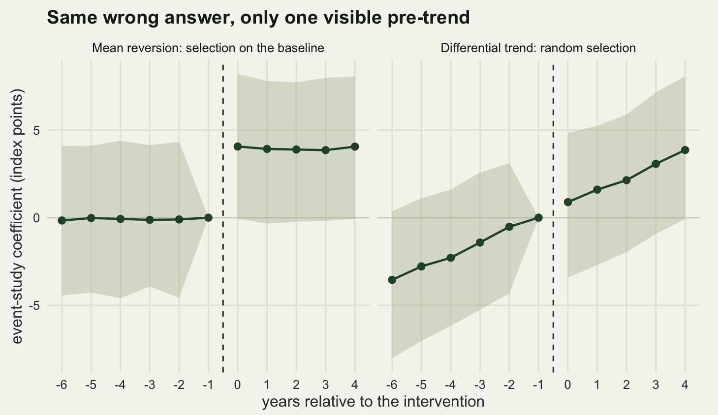
A placebo in time is the other standard check: throw away the post-intervention years, pretend the programme started two years earlier, and re-estimate. The sample-size sweep is the check that settles the matter. If the pre-trend test is merely underpowered, more reaches will wake it up. The sweep below runs both datasets at sample sizes from one hundred to three thousand two hundred reaches and records how often each test rejects.
two_t <- function(v, grp) {
  a <- v[grp == 1]; b <- v[grp == 0]
  est <- mean(a) - mean(b)
  s2 <- ((length(a) - 1) * var(a) + (length(b) - 1) * var(b)) /
        (length(a) + length(b) - 2)
  c(est = est, tstat = est / sqrt(s2 * (1 / length(a) + 1 / length(b))))
}
pre_slope <- function(p) {
  kk <- seq_len(p$npre) - mean(seq_len(p$npre))
  as.vector(p$obs[, seq_len(p$npre), drop = FALSE] %*% kk) / sum(kk^2)
}
plac_time <- function(p) {
  rowMeans(p$obs[, (p$npre - 1):p$npre]) - rowMeans(p$obs[, 1:(p$npre - 2)])
}
diag_row <- function(p, cr) {
  zz <- p$treated
  d <- two_t(post_mean(p) - pre_mean(p), zz)
  s <- two_t(pre_slope(p), zz)
  pl <- two_t(plac_time(p), zz)
  c(d["est"], abs(d["tstat"]) > cr, s["est"], abs(s["tstat"]) > cr,
    pl["est"], abs(pl["tstat"]) > cr)
}

size_grid <- c(100, 200, 400, 800, 1600, 3200)
n_rep_p <- 250
pw <- do.call(rbind, lapply(size_grid, function(ns) {
  cr <- qt(0.975, ns - 2)
  mm <- sapply(seq_len(n_rep_p), function(i)
    c(diag_row(make_panel(200000 + i, ns = ns), cr),
      diag_row(make_panel(300000 + i, ns = ns, rule = "random",
                          drift = drift_cal), cr)))
  data.frame(n = ns,
             mr_did = mean(mm[1, ]), mr_did_rej = mean(mm[2, ]),
             mr_slope_rej = mean(mm[4, ]), mr_plac = mean(mm[5, ]),
             mr_plac_rej = mean(mm[6, ]),
             dt_did = mean(mm[7, ]), dt_did_rej = mean(mm[8, ]),
             dt_slope_rej = mean(mm[10, ]), dt_plac_rej = mean(mm[12, ]))
}))
print(round(pw, 4))
n mr_did mr_did_rej mr_slope_rej mr_plac mr_plac_rej dt_did dt_did_rej
1 100 4.2548 0.540 0.056 -0.1796 0.048 4.0176 0.480
2 200 4.2609 0.836 0.076 -0.2258 0.052 4.1126 0.796
3 400 4.1234 0.972 0.048 0.0087 0.048 4.1035 0.972
4 800 3.9799 1.000 0.048 0.0053 0.024 4.0353 1.000
5 1600 4.1097 1.000 0.048 -0.0665 0.036 4.0082 1.000
6 3200 4.0758 1.000 0.056 -0.0246 0.040 4.0020 1.000
dt_slope_rej dt_plac_rej
1 0.136 0.104
2 0.240 0.168
3 0.388 0.268
4 0.696 0.520
5 0.916 0.792
6 1.000 0.992grab <- function(ns, col) pw[[col]][pw$n == ns]At the design’s own size of 400 reaches the placebo in time returns 0.0087 index points under mean reversion and rejects in 4.8 per cent of replicates; the differential-trend test on the pre-period slope rejects in 4.8 per cent. Both are sitting on their nominal five per cent. Meanwhile the difference-in-differences contrast rejects in 97.2 per cent of replicates, on an effect of zero.
The sample-size column is the part worth keeping. Going from 100 reaches to 3200, the manufactured effect stays at about 4.076 points and the false rejection rate climbs from 54 to 100 per cent, while the pre-trend test stays put: 5.6 per cent at the smallest size and 5.6 per cent at the largest, with the placebo at 4.8 and 4 per cent. On the differential-trend dataset the same two tests go from 13.6 and 10.4 per cent up to 100 and 99.2 per cent. A differential trend is a power problem and a bigger study solves it. Mean reversion is not: there is no pre-trend there to find, and collecting more data only sharpens the confidence interval around the wrong number.
Three analyses of the same table
Three ordinary ways to compare the arms are available in this dataset, and nothing in the data says which to use. The change score subtracts the baseline mean from the post mean and compares the differences, which is the difference-in-differences contrast used above. The raw post-only comparison ignores the baseline; Christie et al (2019) put a number on what that costs across the ecological literature, and the designs that discard the before period come out worst of the set they compared. Analysis of covariance regresses the post value on the treatment indicator with the baseline value as a covariate.
n_rep_l <- 400
lord_run <- function(seed, rule) {
  p <- make_panel(seed, rule = rule)
  bb <- pre_mean(p); pp <- post_mean(p); zz <- p$treated
  m_an <- lm(pp ~ zz + bb)
  c(change = unname(two_t(pp - bb, zz)["est"]),
    postonly = unname(two_t(pp, zz)["est"]),
    ancova = unname(coef(m_an)[2]),
    ancova_se = summary(m_an)$coefficients[2, 2],
    ancova_slope = unname(coef(m_an)[3]),
    quality_gap = mean(p$quality[zz == 1]) - mean(p$quality[zz == 0]))
}
lord_b <- t(sapply(seq_len(n_rep_l), function(i) lord_run(500000 + i, "baseline")))
lord_q <- t(sapply(seq_len(n_rep_l), function(i) lord_run(600000 + i, "quality")))
lord <- rbind(observed_baseline = colMeans(lord_b),
              true_condition = colMeans(lord_q))
print(round(lord, 4))
change postonly ancova ancova_se ancova_slope quality_gap
observed_baseline 4.1289 -12.3680 0.0962 1.2210 0.7556 -12.4435
true_condition -0.0799 -13.6994 -4.4222 1.1119 0.6809 -13.6688print(round(c(ancova_slope_measured = mean(lord_b[, "ancova_slope"]),
ancova_slope_predicted = rel_pre,
ancova_mcse_baseline = sd(lord_b[, "ancova"]) / sqrt(n_rep_l),
change_mcse_quality = sd(lord_q[, "change"]) / sqrt(n_rep_l)), 4)) ancova_slope_measured ancova_slope_predicted ancova_mcse_baseline
0.7556 0.7538 0.0626
change_mcse_quality
0.0546 Under the programme as described, where selection ran on the observed baseline, the three analyses of the same table report 4.129 points for the change score, -12.368 for the post-only comparison, and 0.0962 for the covariance analysis, against a truth of zero. The first says the programme worked, the second says it did serious harm, and the third, with a Monte Carlo standard error of 0.0626 over the replicates, is indistinguishable from nothing having happened. None of them is a coding mistake and all three are computed from identical inputs.
This is Lord’s paradox, which he set out in 1967 as two statisticians reaching opposite conclusions about the same table of weights and neither being able to fault the other’s arithmetic. The resolution is that they answer different questions. The change score asks whether the treated reaches moved more than the untreated ones from wherever each of them started. Covariance analysis asks whether a treated reach ended above an untreated reach that looked the same at baseline. Those coincide only when nothing about the assignment is tangled up in the baseline measurement, and here the assignment is nothing but the baseline measurement. Senn (2006) sets the two estimands against each other and argues that the choice between them belongs to the design rather than to the analyst.
The choice between them is therefore a claim about the assignment mechanism, and the second row of the table shows what happens when that claim changes. There, reaches were selected on their true condition rather than on the monitoring record: an independent habitat survey, say, or a pressure map, with the same administrative term on top. Now the change score returns -0.0799 points, with a Monte Carlo standard error of 0.0546, and covariance analysis returns -4.422. The verdict has swapped ends of the table. Both rows were selected rather than randomised, and what changes between them is whether the rule read the monitoring record or the true condition behind it. Van Breukelen (2006) reports the analogous contrast for randomised against observational studies: covariance analysis is the better of the two under randomisation and the more biased of the two without it.
The mechanism behind the swap is the covariate’s own noise. Where selection ran on the observed baseline the fitted slope is 0.7556, matching the predicted 0.7538, the reliability of the six-year mean; where it ran on the true condition it is 0.6809. Both sit below one: a noisy covariate is only partly adjusted for, so any true difference in condition that is not captured by the observed baseline survives into the treatment coefficient. Glymour et al (2005) trace that residual through in detail and show that adjusting for a noisy baseline can move an estimate away from the truth as easily as towards it. When selection ran on the observed baseline there was no such residual difference, because the baseline was the whole assignment rule. When selection ran on the truth there was, and covariance analysis charged it to the treatment. Both failure modes are the same arithmetic seen from two sides, which is why no diagnostic distinguishes them and why the assignment mechanism has to be written down rather than inferred.
meth <- c("post-only comparison", "change score", "covariance analysis")
mech <- c("Selection on the observed baseline",
          "Selection on the true condition")
fig3 <- data.frame(
  method = factor(rep(meth, 2), levels = meth),
  mechanism = factor(rep(mech, each = 3), levels = mech),
  est = c(lord["observed_baseline", c("postonly", "change", "ancova")],
          lord["true_condition", c("postonly", "change", "ancova")]))
fig3$ok <- ifelse(abs(fig3$est) < 0.5, "unbiased", "biased")

ggplot(fig3, aes(est, method, colour = ok)) +
  geom_vline(xintercept = 0, linetype = "dashed",
             colour = te_pal$ink, linewidth = 0.5) +
  geom_segment(aes(x = 0, xend = est, y = method, yend = method),
               linewidth = 0.6) +
  geom_point(size = 3.4) +
  facet_wrap(~mechanism, ncol = 1) +
  scale_colour_manual(values = c(unbiased = te_pal$forest,
                                 biased = te_pal$clay), guide = "none") +
  scale_x_continuous(expand = expansion(mult = 0.08)) +
  labs(x = "estimated effect (index points), truth is zero",
       y = NULL,
       title = "Which analysis is right depends on how sites were chosen") +
  theme_te() +
  theme(plot.margin = margin(8, 18, 4, 8))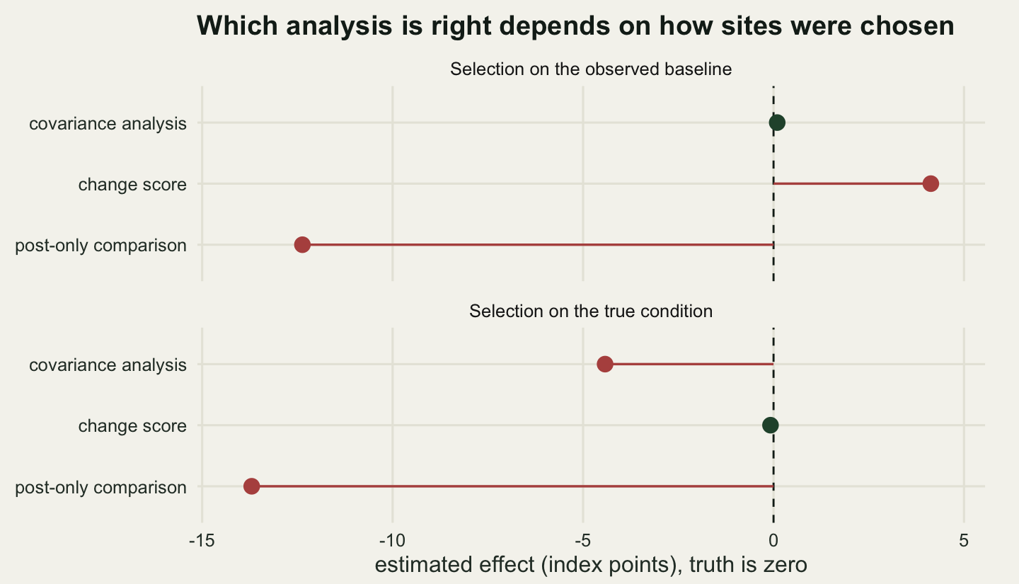
What actually works
Covariance analysis fixed the problem above, but only because the simulation knew that assignment depended on nothing except the baseline value and an independent administrative term. A real programme officer looks at the monitoring record and also at things that are not in it. The design-side repairs are more durable, and there are two of them: change what the selection rule reads, or change which measurement plays the part of the baseline. The sweep below separates them, because they are usually discussed as one recommendation to use more baseline years.
sim_parts <- function(seed, ns = n_site, npre = n_pre, npost = n_post,
                      sd_yr = sd_year, sd_x = 10, rho = 0) {
  set.seed(seed)
  quality <- rnorm(ns, mu_base, sd_site)
  n_yr <- npre + npost
  E <- matrix(0, ns, n_yr)
  E[, 1] <- rnorm(ns, 0, sd_yr)
  if (n_yr > 1) for (j in 2:n_yr)
    E[, j] <- rho * E[, j - 1] + rnorm(ns, 0, sd_yr * sqrt(1 - rho^2))
  list(quality = quality, obs = quality + E,
       admin = rnorm(ns, 0, sd_admin),
       xcov = quality + rnorm(ns, 0, sd_x), npre = npre, npost = npost)
}

run_design <- function(s, sel_idx, base_idx, frac = k_frac, use_x = FALSE) {
  ns <- length(s$quality)
  sc <- if (use_x) s$xcov + s$admin
        else rowMeans(s$obs[, sel_idx, drop = FALSE]) + s$admin
  zz <- rep(0L, ns)
  zz[order(sc)[seq_len(round(ns * frac))]] <- 1L
  bb <- rowMeans(s$obs[, base_idx, drop = FALSE])
  pp <- rowMeans(s$obs[, s$npre + seq_len(s$npost), drop = FALSE])
  c(did = mean((pp - bb)[zz == 1]) - mean((pp - bb)[zz == 0]),
    gap = mean(bb[zz == 0]) - mean(bb[zz == 1]),
    hit = mean(s$quality[zz == 1] <= quantile(s$quality, frac)))
}

n_rep_d <- 250
sims <- lapply(seq_len(n_rep_d), function(i) sim_parts(120000 + i))
avg_over <- function(f) rowMeans(sapply(sims, f))
coef_pred <- function(ms, mb, ov) {
  cv <- sd_year^2 * ov / (ms * mb)
  cv / (sd_site^2 + cv)
}

sweep_both <- do.call(rbind, lapply(seq_len(n_pre), function(m) {
  idx <- (n_pre - m + 1):n_pre
  v <- avg_over(function(s) run_design(s, idx, idx))
  data.frame(years = m, arm = "same years select and compare",
             did = unname(v["did"]), hit = unname(v["hit"]),
             ratio = unname(v["did"] / v["gap"]), pred = coef_pred(m, m, m))
}))
sweep_base <- do.call(rbind, lapply(seq_len(n_pre), function(m) {
  v <- avg_over(function(s) run_design(s, seq_len(n_pre), (n_pre - m + 1):n_pre))
  data.frame(years = m, arm = "select on all six, vary the baseline",
             did = unname(v["did"]), hit = unname(v["hit"]),
             ratio = unname(v["did"] / v["gap"]),
             pred = coef_pred(n_pre, m, m))
}))
num_cols <- c("years", "did", "hit", "ratio", "pred")
print(round(sweep_both[, num_cols], 4))
years did hit ratio pred
1 1 18.1470 0.4506 0.6650 0.6622
2 2 10.6236 0.5094 0.4990 0.4949
3 3 7.5583 0.5380 0.3984 0.3952
4 4 5.9438 0.5532 0.3342 0.3289
5 5 4.8940 0.5656 0.2876 0.2816
6 6 4.1782 0.5744 0.2537 0.2462print(round(sweep_base[, num_cols], 4)) years did hit ratio pred
1 1 4.1032 0.5744 0.2503 0.2462
2 2 4.2088 0.5744 0.2551 0.2462
3 3 4.1569 0.5744 0.2528 0.2462
4 4 4.1729 0.5744 0.2535 0.2462
5 5 4.1906 0.5744 0.2543 0.2462
6 6 4.1782 0.5744 0.2537 0.2462Reading the first table down the years column: selecting and comparing on a single year gives a manufactured effect of 18.147 index points, which is 1.81 times the true standard deviation between reaches. Six years brings it down to 4.178, a reduction of 76.98 per cent, and the measured ratio tracks the predicted noise share at every step, 0.665 against 0.6622 at one year and 0.2537 against 0.2462 at six. More baseline years helps a great deal and does not finish the job.
The second table is the one that separates the two levers. Selection is fixed on all 6 pre-intervention years and only the baseline value changes, from the last year alone to the full six-year mean. The manufactured effect is 4.1032 with one baseline year and 4.1782 with six, a spread of 0.1056 points across the whole column. Averaging more years into the baseline value changes nothing that matters once the selection rule has already read them. What the first table measured was never the length of the baseline average. It was how much noise the selection rule was allowed to see.
split_pt <- n_pre / 2
fix_split <- avg_over(function(s)
  run_design(s, seq_len(split_pt), split_pt + seq_len(split_pt)))
fix_lastyr <- avg_over(function(s)
  run_design(s, seq_len(n_pre - 1), n_pre))
fix_cov <- avg_over(function(s)
  run_design(s, seq_len(n_pre), seq_len(n_pre), use_x = TRUE))
ref_all <- avg_over(function(s)
  run_design(s, seq_len(n_pre), seq_len(n_pre)))

sims_ar <- lapply(seq_len(n_rep_d), function(i) sim_parts(130000 + i, rho = 0.5))
avg_ar <- function(f) rowMeans(sapply(sims_ar, f))
ar_split <- avg_ar(function(s)
  run_design(s, seq_len(split_pt), split_pt + seq_len(split_pt)))
ar_ref <- avg_ar(function(s) run_design(s, seq_len(n_pre), seq_len(n_pre)))

fixes <- rbind(select_and_compare_on_all_six = ref_all,
               select_on_first_three_compare_on_last_three = fix_split,
               select_on_first_five_compare_on_year_six = fix_lastyr,
               select_on_an_external_covariate = fix_cov,
               split_years_with_ar1_noise = ar_split,
               all_six_with_ar1_noise = ar_ref)
print(round(fixes, 4))
did gap hit
select_and_compare_on_all_six 4.1782 16.4670 0.5744
select_on_first_three_compare_on_last_three 0.1388 11.4799 0.5330
select_on_first_five_compare_on_year_six 0.0826 12.1613 0.5646
select_on_an_external_covariate 0.0423 10.6431 0.5014
split_years_with_ar1_noise 2.9810 13.6152 0.4925
all_six_with_ar1_noise 7.0869 19.7799 0.5274print(round(c(hit_cost_of_split = ref_all["hit"] - fix_split["hit"],
hit_cost_of_covariate = ref_all["hit"] - fix_cov["hit"],
ar1_residual_share_of_naive =
ar_split["did"] / ar_ref["did"]), 4)) hit_cost_of_split.hit hit_cost_of_covariate.hit
0.0413 0.0730
ar1_residual_share_of_naive.did
0.4206 Two repairs remove the artefact outright. Selecting on the first 3 pre-intervention years and using the last 3 as the baseline value leaves 0.1388 points; selecting on the first 5 and comparing against year 6 alone leaves 0.0826. That second one is worth pausing on, because it uses a single baseline year, the thing the first table said was worst. The noise in a baseline value only matters if the selection rule saw it. Selecting on a variable that is not the outcome at all, a habitat or pressure covariate correlated with true condition, gives 0.0423.
Neither repair is free, and the price is targeting accuracy. Of the reaches treated under the naive rule, 57.44 per cent are genuinely in the worst fifth by true condition. The split-years rule finds 53.3 per cent and the external covariate 50.14 per cent, so the covariate rule places 7.3 percentage points fewer of its treatments where they were most needed. That is the trade the programme is making: a rule that can be evaluated against one that hits harder.
The split also has a condition attached that is easy to miss. It works because the year-to-year departures are independent, so noise in the first three years carries no information about noise in the last three. Repeating it with an autocorrelated series, a run of dry years rather than independent ones, leaves 2.981 points, which is 42.06 per cent of what the naive rule produces on the same series. Better, and not zero.
fig4 <- rbind(sweep_both[, c("years", "arm", "did")],
              sweep_base[, c("years", "arm", "did")])
fig4$arm <- factor(fig4$arm,
                   levels = c("same years select and compare",
                              "select on all six, vary the baseline"))

ggplot(fig4, aes(years, did, colour = arm, shape = arm)) +
  geom_hline(yintercept = unname(fix_split["did"]), linetype = "dashed",
             colour = te_pal$ink, linewidth = 0.5) +
  annotate("text", x = 3.5, y = unname(fix_split["did"]) + 0.9,
           label = "select and compare on different years",
           hjust = 0, size = 3.1, colour = te_pal$ink) +
  geom_line(linewidth = 0.75) +
  geom_point(size = 2.4) +
  scale_x_continuous(breaks = seq_len(n_pre)) +
  scale_y_continuous(limits = c(0, NA)) +
  scale_colour_manual(values = c(te_pal$clay, te_pal$forest), name = NULL) +
  scale_shape_manual(values = c(16, 15), name = NULL) +
  labs(x = "number of pre-intervention years used",
       y = "manufactured effect (index points)",
       title = "Only the selection rule's noise matters") +
  theme_te() +
  theme(legend.position = "bottom", plot.margin = margin(8, 14, 4, 8))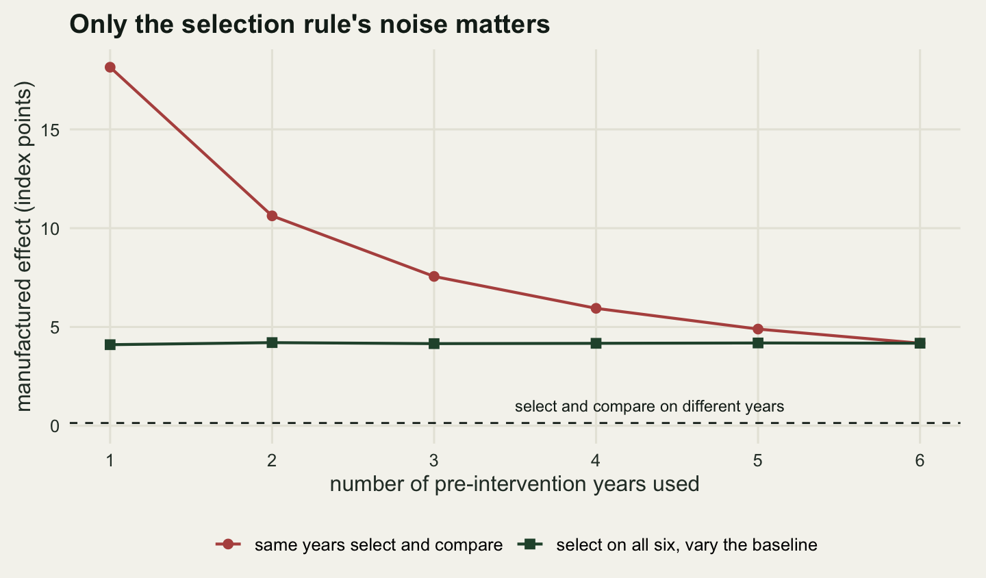
What to take away
Targeting the worst sites is the right thing to do with a restoration budget and it puts a bias into the evaluation that nothing downstream can remove. In the programme simulated here it was worth 4.03 index points, 0.403 times the true standard deviation between reaches, on a treatment that did nothing. The size of it follows a formula with two terms you already have: the noise share of the baseline value, and the observed baseline gap between the arms. Multiply them together before the follow-up survey and you have the number your evaluation will report if the treatment is inert.
The measurement that matters most is the one about diagnostics. Under mean reversion the event-study leads were flat to within 0.1604 index points, the placebo in time returned 0.0087, and both tests rejected at their nominal rate at every sample size from 100 to 3200 reaches, ending at 5.6 and 4 per cent, while the spurious effect itself reached 100 per cent certainty. On a differential-trend dataset calibrated to return the same estimate the same two tests reached 100 and 99.2 per cent. A parallel-trends check is a real check against a trend and it is silent here, because selection on a multi-year average shifts every pre-intervention year by the same amount and a diagnostic built on differences between those years has nothing to work with.
Two results went against what I set up expecting. Selection intensity turned out to be almost irrelevant: going from the worst half to the worst twentieth multiplied the artefact by 1.332 while a change in the noise share multiplied it by 8.701. And lengthening the baseline average, the standard recommendation, does nothing on its own: with selection fixed on all 6 years, moving the baseline value from one year to six changed the artefact by 0.1056 points. What the apparent benefit of long baselines was really measuring is how much noise the selection rule reads, and the cheapest way to cut that to zero is to select on years the comparison does not use: 0.0826 points from a design with a single baseline year in it.
The honest limit sits in the first paragraph of the post. With one baseline observation there is no way to tell a reach that is genuinely poor from one that had a bad year, and nothing in the post-treatment data settles it: the change score, the covariance analysis and the post-only contrast returned 4.129, 0.0962 and -12.368 from identical inputs, and which of the three is unbiased flipped when the assignment mechanism changed while the data looked much the same. The information has to come from before the intervention: more pre-intervention years, a selection rule that reads a different variable from the one the evaluation compares, or at the very least a rule written down in advance so that a reader can work out which of the three answers applies. The design decision and the analysis decision are the same decision, and only one of them can be made after the data arrive.
References
Barnett AG, van der Pols JC, Dobson AJ 2005 International Journal of Epidemiology 34(1):215-220 (10.1093/ije/dyh299)
Kelly C, Price TD 2005 The American Naturalist 166(6):700-707 (10.1086/497402)
Lord FM 1967 Psychological Bulletin 68(5):304-305 (10.1037/h0025105)
Senn S 2006 Statistics in Medicine 25(24):4334-4344 (10.1002/sim.2682)
Van Breukelen GJP 2006 Journal of Clinical Epidemiology 59(9):920-925 (10.1016/j.jclinepi.2006.02.007)
Glymour MM, Weuve J, Berkman LF, Kawachi I, Robins JM 2005 American Journal of Epidemiology 162(3):267-278 (10.1093/aje/kwi187)
Ashenfelter O 1978 The Review of Economics and Statistics 60(1):47-57 (10.2307/1924332)
Larsen AE, Meng K, Kendall BE 2019 Methods in Ecology and Evolution 10(7):924-934 (10.1111/2041-210X.13190)
Christie AP, Amano T, Martin PA, Shackelford GE, Simmons BI, Sutherland WJ 2019 Journal of Applied Ecology 56(12):2742-2754 (10.1111/1365-2664.13499)