library(ggplot2)

te_pal <- list(forest = "#275139", green = "#2f8f63", sage = "#93a87f",
               clay = "#b5534e", gold = "#cda23f", line = "#dad9ca",
               ink = "#16241d", paper = "#f5f4ee")

theme_te <- function() {
  theme_minimal(base_size = 12) +
    theme(panel.grid.minor = element_blank(),
          panel.grid.major = element_line(colour = "#e7e6dc"),
          plot.background = element_rect(fill = "#f5f4ee", colour = NA),
          panel.background = element_rect(fill = "#f5f4ee", colour = NA),
          plot.title = element_text(face = "bold", colour = te_pal$ink),
          axis.title = element_text(colour = "#2c3a31"))
}Restoration trajectories and recovery
R
conservation
restoration
community ecology
ecology tutorial
ggplot2
Measure how far a restored site has recovered in R: metric choice, chronosequence bias, a drifting reference and the trouble with extrapolating an asymptote.
A restoration project reports that the site has recovered most of the way to its reference. The number is doing a lot of work: it goes into a report to a funder, it decides whether a management contract is renewed, and in aggregate it becomes evidence about whether restoration works at all. Underneath it sits a simple arithmetic, the distance the site has travelled from its degraded state divided by the distance it had to travel to reach the reference. Everything difficult is in the two ends of that fraction and in how the middle was measured.
Three decisions fix the answer before the data are collected. The first is which metric goes into the fraction, because species richness, biomass and species composition recover at different speeds on the same ground. The second is what plays the part of the reference, and whether that reference is a set of numbers from an archive or a set of plots surveyed this summer. The third is whether recovery was watched through time on the same sites or reconstructed by lining up sites of different ages, which is a different study answering a slightly different question.
This post builds each of those three in a simulator where the truth is known, and measures how far each one moves the reported recovery. The reference-site logic is the same logic as in Before-after-control-impact designs, and reading that first will help: a reference site is a control, and it earns its place by absorbing the changes that would have happened anyway. The last section takes the assumption that the whole exercise rests on, that the site is heading towards the reference at all, and simulates a site that is not, which is the world of Priority effects and alternative stable states.
Nothing here is quoted from a rule of thumb. Every bias, every threshold and every tolerance is measured in the same simulator, against a truth that we set.
One site, three metrics, three answers
Recovery completeness is the restored value minus the degraded value, divided by the reference value minus the degraded value. It is zero at the moment of intervention and one when the site is indistinguishable from the reference, and it is dimensionless, which is what lets people average it across metrics and across projects.
The simulator below gives every site a trajectory that approaches the reference exponentially, at a rate that differs between metrics and between sites. Species richness recovers quickly because the common species arrive first and there are not many species to find. Vegetation cover follows, because biomass accumulates on a schedule set by growth rather than by dispersal. Compositional similarity to the reference is the slow one, because the last species to arrive are the ones with poor dispersal and narrow requirements, and they are the ones that make a community look like the reference rather than like any old assemblage of survivors.
Each site also gets its own rate multiplier and its own starting condition, so no two sites follow the same curve. The reference and degraded ends of the fraction are estimated from plots, not assumed, because in a real project they are.
set.seed(20260720)

n_site <- 40
n_ref <- 12
n_deg <- 12
report_ages <- c(10, 25, 50)
age_grid <- seq(0, 60, by = 1)

half_time <- c(richness = 7, cover = 18, composition = 55)
deg_level <- c(richness = 8, cover = 15, composition = 0.12)
ref_level <- c(richness = 32, cover = 78, composition = 0.86)
plot_sd   <- c(richness = 2.2, cover = 6, composition = 0.06)
metrics <- names(half_time)

rate_i <- exp(rnorm(n_site, 0, 0.25))
start_i <- rnorm(n_site, 0, 0.05)

dat <- do.call(rbind, lapply(metrics, function(m) {
  kk <- log(2) / half_time[[m]]
  gr <- expand.grid(site = seq_len(n_site), age = age_grid)
  cc <- 1 - (1 - start_i[gr$site]) * exp(-kk * rate_i[gr$site] * gr$age)
  data.frame(metric = m, site = gr$site, age = gr$age, truth = cc,
             value = deg_level[[m]] + (ref_level[[m]] - deg_level[[m]]) * cc +
               rnorm(nrow(gr), 0, plot_sd[[m]]))
}))

ref_mean <- sapply(metrics, function(m) mean(rnorm(n_ref, ref_level[[m]], plot_sd[[m]])))
deg_mean <- sapply(metrics, function(m) mean(rnorm(n_deg, deg_level[[m]], plot_sd[[m]])))

dat$completeness <- (dat$value - deg_mean[dat$metric]) /
  (ref_mean[dat$metric] - deg_mean[dat$metric])
site_mean <- aggregate(completeness ~ metric + age, dat, mean)

comp_tab <- sapply(report_ages, function(a)
  sapply(metrics, function(m)
    100 * site_mean$completeness[site_mean$metric == m & site_mean$age == a]))
colnames(comp_tab) <- paste0("year_", report_ages)
print(round(comp_tab, 1))
year_10 year_25 year_50
richness 66.1 93.5 101.5
cover 36.6 66.1 92.2
composition 13.6 29.5 52.1print(round(c(sites = n_site, reference_plots = n_ref, degraded_plots = n_deg,
half_richness = half_time[["richness"]],
half_cover = half_time[["cover"]],
half_composition = half_time[["composition"]]), 1)) sites reference_plots degraded_plots half_richness
40 12 12 7
half_cover half_composition
18 55 print(round(apply(comp_tab, 2, function(z) max(z) / min(z)), 2))year_10 year_25 year_50
4.86 3.17 1.95 print(round(c(deg_richness = deg_level[["richness"]], ref_richness = ref_level[["richness"]],
deg_cover = deg_level[["cover"]], ref_cover = ref_level[["cover"]],
deg_similarity = deg_level[["composition"]],
ref_similarity = ref_level[["composition"]]), 2)) deg_richness ref_richness deg_cover ref_cover deg_similarity
8.00 32.00 15.00 78.00 0.12
ref_similarity
0.86 Forty restored sites, twelve reference plots and twelve degraded plots. At ten years the same sites are 66.1 per cent recovered in richness, 36.6 per cent in cover and 13.6 per cent in composition. The fastest metric divides the slowest by 4.86. At twenty-five years the three values are 93.5, 66.1 and 29.5 per cent, a ratio of 3.17, and at fifty years they are 101.5, 92.2 and 52.1 per cent, a ratio of 1.95.
Every one of those numbers is correct. Each is the honest answer to the question “how far towards the reference is this site” for one currency of measurement. A project that reports the richness number at ten years is reporting 66.1 per cent, and a project that reports the composition number at the same visit on the same plots is reporting 13.6 per cent, and neither is lying. The headline is a choice, and the spread it hides is more than fourfold in the first decade.
At fifty years the richness figure is 101.5 per cent, and on some runs it goes past a hundred. That is not a bug. Restored sites can carry more species than mature reference sites, because they hold a mix of colonists and residents while the reference has settled into whatever the site supports at equilibrium. Richness is not a monotone function of ecological condition, and this is the reason a richness target is the easiest of all the targets to hit.
lab_metric <- c(richness = "Species richness", cover = "Vegetation cover",
                composition = "Similarity to reference")
dat$label <- factor(lab_metric[dat$metric], levels = lab_metric)
site_mean$label <- factor(lab_metric[site_mean$metric], levels = lab_metric)

ggplot(dat, aes(age, truth, colour = label)) +
  geom_hline(yintercept = 1, colour = te_pal$ink, linetype = "22", linewidth = 0.5) +
  geom_vline(xintercept = report_ages, colour = te_pal$line, linewidth = 0.6) +
  geom_line(aes(group = interaction(site, metric)), linewidth = 0.3, alpha = 0.3) +
  geom_line(data = site_mean, aes(age, completeness, colour = label), linewidth = 1.2) +
  scale_colour_manual(values = c(te_pal$forest, te_pal$gold, te_pal$clay), name = NULL) +
  coord_cartesian(ylim = c(-0.1, 1.25)) +
  labs(x = "Years since restoration", y = "Recovery completeness",
       title = "Three metrics, three answers on the same sites") +
  theme_te() +
  theme(legend.position = "top")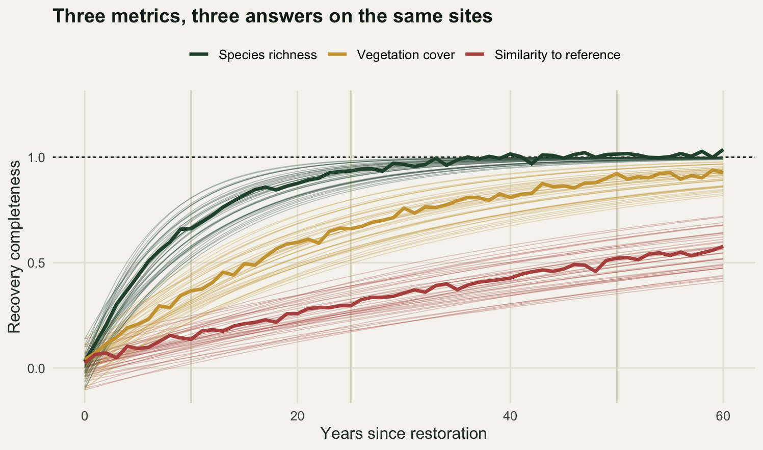
Space for time, and the land that was chosen
Waiting fifty years for an answer is not an option, so the common substitute is a chronosequence: find restorations of many different ages, survey them all in one field season, and read the age axis as if it were time. The substitution is valid when the only thing that differs between an old restoration and a young one is age.
That condition fails in a specific and predictable way. Restoration goes where it is cheap and promising first. Early projects took the fields with intact soil, the wetlands with the ditch still blockable, the sites next to remnant habitat. Later projects, competing for the leftovers, took harder ground. Site age and site quality end up correlated, and the chronosequence reads the resulting difference between old and young sites as the passage of time.
The simulator below puts that correlation in by hand. Each site has a quality offset that raises or lowers its completeness at every age, and the correlation between age and quality is a parameter we can turn. Against it we run the study a chronosequence cannot afford: twenty-four sites, each visited four times over thirty years. The estimator for the repeated measures is the within-site one, which compares each site against its own earlier self and so cannot be fooled by a difference in quality between sites.
k_true <- log(2) / 60
n_chr <- 60
n_panel <- 24
age_lo <- 3; age_hi <- 60
q_sd <- 0.24
obs_sd <- 0.06
rho_base <- 0.6
curve_f <- function(t, k) 1 - exp(-k * t)

fit_k_cross <- function(t, y) {
  obj <- function(lk) sum((y - curve_f(t, exp(lk)))^2)
  exp(optimize(obj, c(log(0.002), log(1)), tol = 1e-10)$minimum)
}
fit_k_within <- function(t, y, id) {
  ybar <- ave(y, id)
  obj <- function(lk) {
    f <- curve_f(t, exp(lk))
    sum(((y - ybar) - (f - ave(f, id)))^2)
  }
  exp(optimize(obj, c(log(0.002), log(1)), tol = 1e-10)$minimum)
}
make_chrono <- function(rho, n = n_chr) {
  age <- runif(n, age_lo, age_hi)
  z <- (age - mean(age)) / sd(age)
  q <- q_sd * (rho * z + sqrt(1 - rho^2) * rnorm(n))
  data.frame(site = seq_len(n), age = age, quality = q,
             y = curve_f(age, k_true) + q + rnorm(n, 0, obs_sd))
}
make_panel <- function(rho, n = n_panel, visits = c(0, 10, 20, 30)) {
  first <- runif(n, age_lo, age_hi - max(visits))
  z <- (first - mean(first)) / sd(first)
  q <- q_sd * (rho * z + sqrt(1 - rho^2) * rnorm(n))
  do.call(rbind, lapply(seq_len(n), function(i) {
    tt <- first[i] + visits
    data.frame(site = i, age = tt, quality = q[i],
               y = curve_f(tt, k_true) + q[i] + rnorm(length(tt), 0, obs_sd))
  }))
}

set.seed(9021)
ch <- make_chrono(rho_base)
pn <- make_panel(rho_base)
k_ch <- fit_k_cross(ch$age, ch$y)
k_pn <- fit_k_within(pn$age, pn$y, pn$site)
print(round(c(chrono_sites = n_chr, panel_sites = n_panel, visits = 4,
              target_correlation = rho_base,
              realised_correlation = cor(ch$age, ch$quality),
              true_half_time = log(2) / k_true,
              chrono_half_time = log(2) / k_ch,
              panel_half_time = log(2) / k_pn,
              chrono_bias_pct = 100 * (k_ch / k_true - 1),
              panel_bias_pct = 100 * (k_pn / k_true - 1)), 3))
chrono_sites panel_sites visits
60.000 24.000 4.000
target_correlation realised_correlation true_half_time
0.600 0.510 60.000
chrono_half_time panel_half_time chrono_bias_pct
46.077 59.610 30.218
panel_bias_pct
0.654 The true half-time of recovery is 60 years. The chronosequence, built from 60 sites spanning ages of three to sixty, returns 46.077 years. The repeated-measures study, built from 24 sites and four visits each, returns 59.61. As a rate, the chronosequence is 30.218 per cent fast and the repeated measures 0.654 per cent fast. The realised correlation between age and quality in this particular draw of sites is 0.51.
The direction is the one that matters for policy. A chronosequence built on sites that were chosen in a sensible order says restoration is faster than it is, which is the answer that gets a scheme extended.
rho_seq <- seq(0, 0.9, by = 0.05)
nrep_rho <- 150
tolerance <- 25
set.seed(77)
bias_rho <- sapply(rho_seq, function(r)
  median(sapply(seq_len(nrep_rho), function(i) {
    d <- make_chrono(r)
    100 * (fit_k_cross(d$age, d$y) / k_true - 1)
  })))
print(round(rbind(correlation = rho_seq, median_bias_pct = bias_rho), 2))
[,1] [,2] [,3] [,4] [,5] [,6] [,7] [,8] [,9] [,10] [,11]
correlation 0.00 0.05 0.10 0.15 0.20 0.25 0.3 0.35 0.40 0.45 0.50
median_bias_pct -0.56 0.82 3.52 4.83 6.61 8.23 11.1 12.75 13.69 14.27 18.25
[,12] [,13] [,14] [,15] [,16] [,17] [,18] [,19]
correlation 0.55 0.60 0.65 0.70 0.75 0.80 0.85 0.90
median_bias_pct 19.01 18.55 22.64 24.09 23.29 24.58 26.93 29.58print(c(replicates = nrep_rho, tolerance_pct = tolerance,
first_correlation = min(rho_seq[bias_rho > tolerance]))) replicates tolerance_pct first_correlation
150.00 25.00 0.85 Sweeping the age-quality correlation from zero to 0.9, with 150 replicate chronosequences at each value, gives the price list. At no correlation the median bias is -0.56 per cent, which is the estimator working. At a correlation of 0.3 it is 11.1 per cent, at 0.5 it is 18.25 per cent, and the first value on the grid at which the median bias exceeds a tolerance of 25 per cent is a correlation of 0.85, where it reaches 26.93 per cent.
Read that carefully, because it cuts both ways. A chronosequence is not ruined by a mild correlation between age and site quality: at 0.3, which is a plausible amount of real-world sorting, the rate is 11 per cent fast, and that is smaller than most of the other uncertainties in a restoration study. It takes a strong correlation to move the rate by a quarter. In this draw, the single chronosequence fitted above came back 30.218 per cent fast at a target correlation of 0.6, where the median across replicates is 18.55 per cent. A single chronosequence carries its own sampling noise on top of the bias, and it is the single chronosequence you will publish.
grid_t <- seq(0, age_hi, by = 0.5)
pan_lab <- c("Chronosequence: one visit to each of sixty sites",
             "Repeated measures: twenty-four sites, four visits")
fits_line <- rbind(
  data.frame(age = grid_t, y = curve_f(grid_t, k_ch), kind = "fitted", panel = pan_lab[1]),
  data.frame(age = grid_t, y = curve_f(grid_t, k_true), kind = "truth", panel = pan_lab[1]),
  data.frame(age = grid_t, y = curve_f(grid_t, k_pn), kind = "fitted", panel = pan_lab[2]),
  data.frame(age = grid_t, y = curve_f(grid_t, k_true), kind = "truth", panel = pan_lab[2]))
fits_line$panel <- factor(fits_line$panel, levels = pan_lab)
ch$panel <- factor(pan_lab[1], levels = pan_lab)
pn$panel <- factor(pan_lab[2], levels = pan_lab)

ggplot(ch, aes(age, y)) +
  geom_line(data = pn, aes(age, y, group = site), colour = te_pal$sage, linewidth = 0.5) +
  geom_point(aes(fill = quality), size = 2.1, shape = 21, stroke = 0.3,
             colour = te_pal$ink) +
  geom_point(data = pn, aes(age, y), colour = te_pal$green, size = 1) +
  geom_line(data = fits_line, aes(age, y, linetype = kind), colour = te_pal$clay,
            linewidth = 0.8) +
  facet_wrap(~panel) +
  scale_fill_gradient(low = "#a9bd93", high = te_pal$forest, name = "Land quality") +
  scale_linetype_manual(values = c(fitted = "solid", truth = "22"), name = NULL) +
  labs(x = "Years since restoration", y = "Recovery completeness",
       title = "Older sites were also better sites") +
  theme_te() +
  theme(legend.position = "top",
        strip.text = element_text(colour = te_pal$ink, face = "bold"))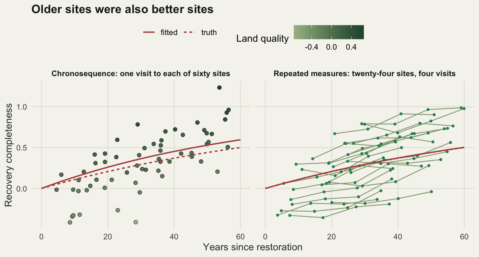
The right-hand panel shows why the within-site estimator survives. Each site’s four visits form a short track, and the tracks sit at different heights because the sites differ in quality, but each track has the slope of the true curve. Height is what the chronosequence sees and slope is what the repeated measures see, and only the slope is recovery.
The reference moves
The second end of the fraction is the reference, and the arithmetic quietly assumes it holds still. It does not. Nitrogen deposition falls, a drought decade arrives, a deer population trebles, a river is cleaned up. Whatever it is, it acts on the reference sites and on the restored sites alike, and a fifty-year study is long enough for it to matter.
There are two defensible ways to handle it and they answer different questions. A fixed historical baseline divides by the reference value as it was at the start, which asks whether the site has reached the state the project set out to create. A contemporaneous reference divides by reference plots surveyed in the same year as the restored plots, which asks whether the site now looks like an intact site looks now. The simulation gives both, on the same restored sites, with a background trend of 0.6 per cent of the reference range per year, run once upward and once downward.
set.seed(5150)
k_ref <- log(2) / 30
drift <- 0.006
n_plot <- 15
ref_sd <- 0.05

sim_year <- function(t, dr) {
  restored <- curve_f(t, k_ref) + dr * t + rnorm(n_plot, 0, ref_sd)
  contemporary <- 1 + dr * t + rnorm(n_plot, 0, ref_sd)
  historical <- rnorm(n_plot, 1, ref_sd)
  c(fixed = mean(restored) / mean(historical),
    contemporaneous = mean(restored) / mean(contemporary))
}
show_ref <- function(m) {
  out <- rbind(m, divergence = m[1, ] - m[2, ],
               convergence_truth = curve_f(report_ages, k_ref))
  colnames(out) <- paste0("year_", report_ages)
  round(100 * out, 1)
}
imp_m <- sapply(report_ages, function(t) sim_year(t, drift))
dec_m <- sapply(report_ages, function(t) sim_year(t, -drift))

print(round(c(reference_plots = n_plot, composition_half_time = log(2) / k_ref,
              drift_pct_of_range_per_year = 100 * drift), 2))
reference_plots composition_half_time
15.0 30.0
drift_pct_of_range_per_year
0.6 print(show_ref(imp_m)) year_10 year_25 year_50
fixed 27.0 60.0 98.7
contemporaneous 25.3 52.2 75.2
divergence 1.7 7.8 23.5
convergence_truth 20.6 43.9 68.5print(show_ref(dec_m)) year_10 year_25 year_50
fixed 15.5 29.1 37.0
contemporaneous 16.8 33.8 53.6
divergence -1.3 -4.7 -16.6
convergence_truth 20.6 43.9 68.5Take the improving reference first, the first of the two tables. Measured against the fixed historical baseline the site is 27.0 per cent recovered at ten years, 60.0 at twenty-five and 98.7 at fifty. Measured against reference plots surveyed in the same year it is 25.3, 52.2 and 75.2 per cent. The truth of convergence, the part of the change that the restoration itself produced, is 20.6, 43.9 and 68.5 per cent. The two measures diverge by 1.7 points at ten years and by 23.5 at fifty.
The fifty-year number is the one to sit with. A project measured against the archive reports 98.7 per cent recovery, which in any report reads as complete success, when the restored site has in fact closed 68.5 per cent of its own gap and the rest of the movement came from a trend that lifted the untouched reference by just as much. Nothing was faked. The baseline was simply left in the past.
Now the declining reference, the second table. Against the fixed baseline the site reports 15.5, 29.1 and 37.0 per cent, and against contemporaneous plots it reports 16.8, 33.8 and 53.6 per cent. The signs of the divergence reverse: -1.3, -4.7 and -16.6 points. Against the archive the project looks like a failure, because the world it was trying to rebuild no longer exists anywhere. Against today’s best remaining sites it looks like a partial success, because the target has come down to meet it.
Neither is the wrong number. They answer different questions, and the questions differ in a way that matters for what happens next. The fixed baseline is the right denominator for asking whether a commitment has been met, and for noticing that the whole system is sliding. The contemporaneous reference is the right denominator for asking whether the intervention worked, because it nets out the change that would have happened anyway, which is exactly the job a control does in a before-after-control-impact design. A monitoring report that gives one without saying which it is has left out the more informative half.
tt_ref <- seq(0, 50, by = 0.5)
kind_lab <- c("Fixed historical baseline", "Contemporaneous reference",
              "Convergence only")
one_side <- function(dr, nm) {
  base <- curve_f(tt_ref, k_ref)
  rbind(
    data.frame(year = tt_ref, y = base + dr * tt_ref, kind = kind_lab[1], side = nm),
    data.frame(year = tt_ref, y = (base + dr * tt_ref) / (1 + dr * tt_ref),
               kind = kind_lab[2], side = nm),
    data.frame(year = tt_ref, y = base, kind = kind_lab[3], side = nm))
}
side_lab <- c("Reference improving", "Reference declining")
ref_long <- rbind(one_side(drift, side_lab[1]), one_side(-drift, side_lab[2]))
ref_long$side <- factor(ref_long$side, levels = side_lab)
ref_long$kind <- factor(ref_long$kind, levels = kind_lab)
ref_pts <- rbind(
  data.frame(year = report_ages, y = imp_m[1, ], kind = kind_lab[1], side = side_lab[1]),
  data.frame(year = report_ages, y = imp_m[2, ], kind = kind_lab[2], side = side_lab[1]),
  data.frame(year = report_ages, y = dec_m[1, ], kind = kind_lab[1], side = side_lab[2]),
  data.frame(year = report_ages, y = dec_m[2, ], kind = kind_lab[2], side = side_lab[2]))
ref_pts$side <- factor(ref_pts$side, levels = side_lab)
ref_pts$kind <- factor(ref_pts$kind, levels = kind_lab)

ggplot(ref_long, aes(year, y, colour = kind)) +
  geom_hline(yintercept = 1, colour = te_pal$ink, linetype = "22", linewidth = 0.5) +
  geom_line(linewidth = 0.9) +
  geom_point(data = ref_pts, size = 2.4) +
  facet_wrap(~side) +
  scale_colour_manual(values = c(te_pal$clay, te_pal$forest, te_pal$sage), name = NULL) +
  labs(x = "Years since restoration", y = "Recovery completeness",
       title = "Two references, two verdicts") +
  theme_te() +
  theme(legend.position = "top",
        strip.text = element_text(colour = te_pal$ink, face = "bold"))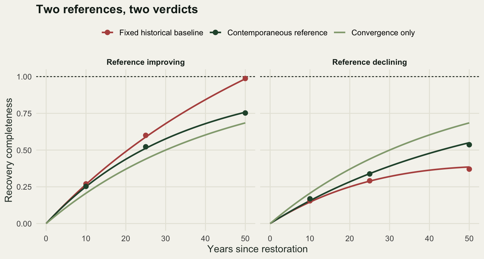
Extrapolating the asymptote
A fourth habit is to fit a saturating curve to the years of monitoring that exist and read off two things the data do not contain: the level the site will eventually reach, and the year it will get there. The model is the same exponential approach, now with the ceiling estimated rather than fixed at the reference:
\[C(t) = A \left( 1 - e^{-kt} \right)\]
with \(A\) the asymptote and \(k\) the rate. Fitting it is easy, because for any candidate rate the asymptote follows in closed form by least squares, leaving a one-dimensional search. The difficulty is not numerical.
The system below has a true half-time of 45 years, so the true time to reach 90 per cent of the reference is 149.49 years. We survey it every two years, truncate the record at ten, twenty and forty years, and fit the same model to each piece of the same series.
k_slow <- log(2) / 45
t90_true <- log(10) / k_slow
survey_sd <- 0.05
survey_gap <- 2

fit_sat <- function(t, y) {
  obj <- function(lk) {
    x <- 1 - exp(-exp(lk) * t)
    aa <- sum(x * y) / sum(x * x)
    sum((y - aa * x)^2)
  }
  lo <- log(0.0015); hi <- log(0.6)
  op <- optimize(obj, c(lo, hi), tol = 1e-11)
  kk <- exp(op$minimum)
  x <- 1 - exp(-kk * t)
  aa <- sum(x * y) / sum(x * x)
  list(k = kk, a = aa, rss = op$objective, t90 = log(10) / kk,
       edge = as.numeric(op$minimum <= lo + 1e-6 || op$minimum >= hi - 1e-6),
       resid_sd = sqrt(op$objective / max(length(t) - 2, 1)))
}
sim_slow <- function(len) {
  tt <- seq(survey_gap, len, by = survey_gap)
  data.frame(t = tt, y = curve_f(tt, k_slow) + rnorm(length(tt), 0, survey_sd))
}

set.seed(2211)
full_series <- sim_slow(40)
record_lens <- c(10, 20, 40)
trunc_list <- lapply(record_lens, function(L) {
  d <- full_series[full_series$t <= L, ]
  c(fit_sat(d$t, d$y), list(record = L, surveys = nrow(d)))
})
trunc_fits <- do.call(rbind, lapply(trunc_list, function(f)
  data.frame(record = f$record, surveys = f$surveys, asymptote = f$a, t90 = f$t90,
             t90_error_pct = 100 * (f$t90 / t90_true - 1), at_edge = f$edge)))
print(round(trunc_fits, 2))
record surveys asymptote t90 t90_error_pct at_edge
1 10 5 12.74 1535.06 926.88 1
2 20 10 0.30 27.37 -81.69 0
3 40 20 1.14 163.76 9.55 0print(round(c(true_half_time = log(2) / k_slow, true_asymptote = 1,
true_t90 = t90_true, survey_sd = survey_sd,
survey_interval = survey_gap), 2)) true_half_time true_asymptote true_t90 survey_sd survey_interval
45.00 1.00 149.49 0.05 2.00 One site, one series, three places to stop reading it. Ten years of data give an asymptote of 12.74 and a time to 90 per cent recovery of 1535.06 years, 926.9 per cent off the truth. Twenty years give 0.3 and 27.37 years, -81.7 per cent off. Forty years give 1.14 and 163.76 years, 9.5 per cent off. Where the last column carries a flag the fit has run to the edge of the searched rate interval and is not an estimate at all: a short stretch of a saturating curve is close enough to a straight line that the model cannot find the curvature, so it answers with either a site that will keep improving forever or one that has already finished.
The two short answers are wrong by tens or hundreds of per cent, and they need not even agree on the direction: one can say the site will overshoot the reference several times over and needs centuries, the other that it will never get close and has already stopped. Both were fitted to the same site, by the same code, from nested subsets of one series.
set.seed(4242)
nrep_len <- 300
len_seq <- seq(10, 100, by = 10)
trunc_sweep <- as.data.frame(t(sapply(len_seq, function(L) {
  z <- t(sapply(seq_len(nrep_len), function(i) {
    d <- sim_slow(L)
    f <- fit_sat(d$t, d$y)
    c(f$a, f$t90)
  }))
  c(record = L, median_asymptote = median(z[, 1]), median_t90 = median(z[, 2]),
    median_error_pct = 100 * (median(z[, 2]) / t90_true - 1),
    t90_q10 = as.numeric(quantile(z[, 2], 0.1)),
    t90_q90 = as.numeric(quantile(z[, 2], 0.9)),
    frac_within_25 = mean(abs(z[, 2] / t90_true - 1) <= 0.25),
    frac_too_fast = mean(z[, 2] < t90_true))
})))
print(round(trunc_sweep, 2))
record median_asymptote median_t90 median_error_pct t90_q10 t90_q90
1 10 0.91 123.50 -17.38 6.55 1535.06
2 20 0.91 128.28 -14.18 29.78 1535.06
3 30 1.11 163.92 9.66 56.50 1535.06
4 40 1.05 158.33 5.92 81.37 794.48
5 50 1.07 160.82 7.58 98.29 347.68
6 60 0.99 148.67 -0.54 110.51 240.91
7 70 0.99 147.64 -1.24 116.21 205.36
8 80 1.00 148.54 -0.64 121.80 188.53
9 90 1.00 148.66 -0.56 126.24 178.11
10 100 1.01 149.69 0.14 128.65 174.28
frac_within_25 frac_too_fast
1 0.03 0.51
2 0.09 0.52
3 0.20 0.46
4 0.33 0.46
5 0.45 0.43
6 0.63 0.51
7 0.75 0.53
8 0.86 0.51
9 0.91 0.52
10 0.96 0.49half_ok <- min(trunc_sweep$record[trunc_sweep$frac_within_25 >= 0.5])
print(round(c(replicates = nrep_len,
first_median_within = min(trunc_sweep$record[
abs(trunc_sweep$median_error_pct) <= tolerance]),
first_half_within = half_ok,
share_of_true_t90 = half_ok / t90_true), 3)) replicates first_median_within first_half_within share_of_true_t90
300.000 10.000 60.000 0.401 Repeating the exercise 300 times at each record length turns the anecdote into a distribution, and the distribution behaves differently from its own centre. On this run the median estimate at ten years is -17.4 per cent off the truth, and from thirty years on the median sits within about ten per cent at every length on the grid. The median settles fast, and judged on it alone you would conclude that a few decades of monitoring is plenty.
The individual estimate says otherwise. At a ten-year record only 0.03 of replicates land within 25 per cent of the true recovery time, and the middle 80 per cent of estimates runs from 6.55 years to 1535.06, where that upper figure is the edge of the searched rate interval rather than a fitted number, the same non-answer a truncated record can produce. At twenty years it is 0.09 of replicates, at forty years 0.33, and the shortest record on the grid at which at least half the replicates come within 25 per cent is 60 years, which is 0.401 of the true recovery time itself. To estimate when a site will be 90 per cent recovered you need to have watched it for something like the first two fifths of that period.
That was not what I expected to find, and the two criteria disagreeing is the useful part. The median of a heavy-tailed distribution is a poor summary of what one study will report, and a simulation that only checks the median will pronounce a short record adequate.
The direction of the bias needs stating precisely, because it is not a simple one. The fraction of replicates that come back too fast is 0.51 at ten years and stays near a half at every length, so the sign of the error is not where the problem lies. The lean is in the shape: the errors that are too fast are bounded, because a recovery time cannot be less than zero, and the errors that are too slow are not. The ceiling is no steadier. The median asymptote at ten and twenty years is 0.91 and 0.91 against a true value of one, and repeating the whole exercise on fresh data drops those medians on either side of one. A short record does not pin down where the site is going any more than it pins down when it will get there.
What the trajectory cannot tell you
Everything above assumes the site is converging on the reference. Recovery completeness is only meaningful as a fraction of a journey if the destination is where the site is going, and the curve-fitting only makes sense if the shape is saturating. Neither is guaranteed. A site can cross into an alternative state, held there by an invader, a shifted nutrient regime, or a feedback that the original community used to suppress, and once there it is not slowly recovering at all.
The site simulated below is identical to a genuinely recovering site for its first twelve years. Then an invader establishes and the trajectory turns over. The comparison site has a half-time of 8.3 years and converges on the reference in the ordinary way.
k_rec <- 0.0835
t_switch <- 12
drop_size <- 0.75
drop_rate <- 0.07
rec_path <- function(t) curve_f(t, k_rec)
alt_path <- function(t) rec_path(t) -
  drop_size * (1 - exp(-drop_rate * pmax(0, t - t_switch)))

print(round(c(recovering_half_time = log(2) / k_rec, switch_year = t_switch,
              alt_year_10 = 100 * alt_path(10), alt_year_25 = 100 * alt_path(25),
              alt_year_50 = 100 * alt_path(50),
              recovering_year_10 = 100 * rec_path(10),
              recovering_year_50 = 100 * rec_path(50),
              alt_peak = 100 * max(alt_path(seq(0, 80, by = 0.5)))), 2))
recovering_half_time switch_year alt_year_10
8.30 12.00 56.61
alt_year_25 alt_year_50 recovering_year_10
42.79 28.71 56.61
recovering_year_50 alt_peak
98.46 63.29 set.seed(808)
t10 <- seq(survey_gap, 10, by = survey_gap)
y_alt10 <- alt_path(t10) + rnorm(length(t10), 0, survey_sd)
y_rec10 <- rec_path(t10) + rnorm(length(t10), 0, survey_sd)
f_alt <- fit_sat(t10, y_alt10)
f_rec <- fit_sat(t10, y_rec10)
print(round(c(surveys = length(t10), asymptote_alt = f_alt$a,
asymptote_recovering = f_rec$a, t90_alt = f_alt$t90,
t90_recovering = f_rec$t90, resid_sd_alt = f_alt$resid_sd,
resid_sd_recovering = f_rec$resid_sd,
resid_sd_gap = abs(f_alt$resid_sd - f_rec$resid_sd)), 4)) surveys asymptote_alt asymptote_recovering
5.0000 0.5940 1.0974
t90_alt t90_recovering resid_sd_alt
11.5040 33.9655 0.0756
resid_sd_recovering resid_sd_gap
0.0705 0.0051 At ten years the alternative-state site is 56.61 per cent recovered, which in a monitoring report is good progress: over half way in a decade. At twenty-five years it is 42.79 per cent and at fifty years it is 28.71 per cent. It peaked at 63.29 per cent in year twelve and has been losing ground ever since. The completeness figure at ten years was not wrong. It was a correct measurement of a quantity that had stopped meaning what its name says.
The ten-year fits are the point. On this pair of noisy records the alternative-state site returns an asymptote of 0.594 and the genuinely recovering site returns 1.0974, with residual standard deviations of 0.0756 and 0.0705, a gap of 0.0051. The fits are equally good. The difference in the asymptote looks large until you ask what a ten-year record can resolve.
set.seed(1234)
nrep_sep <- 300
sep_tab <- do.call(rbind, lapply(seq(10, 30, by = 2), function(L) {
  ts <- seq(survey_gap, L, by = survey_gap)
  mc <- t(sapply(seq_len(nrep_sep), function(i)
    c(fit_sat(ts, alt_path(ts) + rnorm(length(ts), 0, survey_sd))$a,
      fit_sat(ts, rec_path(ts) + rnorm(length(ts), 0, survey_sd))$a)))
  data.frame(record = L, median_alt = median(mc[, 1]),
             median_recovering = median(mc[, 2]),
             alt_below_5th = mean(mc[, 1] < quantile(mc[, 2], 0.05)),
             alt_lower = mean(mc[, 1] < mc[, 2]),
             rec_q05 = as.numeric(quantile(mc[, 2], 0.05)),
             rec_q95 = as.numeric(quantile(mc[, 2], 0.95)))
}))
print(round(sep_tab, 3))
record median_alt median_recovering alt_below_5th alt_lower rec_q05 rec_q95
1 10 0.954 1.001 0.033 0.527 0.591 39.426
2 12 1.009 0.998 0.050 0.490 0.657 2.644
3 14 0.789 0.993 0.307 0.803 0.726 1.907
4 16 0.674 1.003 0.960 0.983 0.794 1.546
5 18 0.618 1.014 1.000 1.000 0.828 1.400
6 20 0.588 1.013 1.000 1.000 0.857 1.251
7 22 0.559 1.000 1.000 1.000 0.878 1.228
8 24 0.539 1.004 1.000 1.000 0.893 1.171
9 26 0.522 1.012 1.000 1.000 0.913 1.134
10 28 0.508 0.996 1.000 1.000 0.916 1.106
11 30 0.495 1.002 1.000 1.000 0.928 1.108print(c(replicates = nrep_sep,
first_separating = min(sep_tab$record[sep_tab$alt_below_5th >= 0.5]))) replicates first_separating
300 16 Across 300 replicate pairs of ten-year records, the median fitted asymptote is 0.954 for the alternative-state site and 1.001 for the recovering one, and the alternative-state site’s asymptote is the lower of the pair in 0.527 of replicates, which is a coin toss. The middle 90 per cent of asymptotes fitted to ten-year records from the genuinely recovering site runs from 0.591 to 39.426. On this pair of records the single fit of 0.594 above sits at the bottom edge of that range: it is an ordinary draw from the noise, not a signal. Judged against the recovering site’s own fifth percentile, the alternative-state site is flagged in 0.033 of replicates, which is what a five per cent rule does when there is nothing to find.
There is nothing to find because for the first twelve years the two sites are the same process. No diagnostic can separate distributions that are identical, and no amount of care with the curve fitting will change that. What does change it is more years. Extending the record to fourteen years flags the alternative-state site in 0.307 of replicates, and at sixteen years, four years past the switch and two surveys into the decline, it is 0.96. The first record length on the grid at which the majority of replicates separate is 16 years.
That is the honest limit of the whole apparatus, and it is not a caveat about statistical power. Recovery completeness, the fitted trajectory and the extrapolated asymptote all presuppose that the reference is the right destination and that the site is travelling towards it. The data available in the early years of a project cannot test either presupposition. They can only be tested by continuing to measure, past the point where the reporting cycle has already recorded the project as a success.
tt_long <- seq(0, 200, by = 1)
pan2 <- c("One converging site, three record lengths",
          "Two sites, one identical decade")
left <- do.call(rbind, lapply(trunc_list, function(f)
  data.frame(t = tt_long, y = f$a * (1 - exp(-f$k * tt_long)),
             series = paste(f$record, "year record"), panel = pan2[1])))
left <- rbind(left, data.frame(t = tt_long, y = curve_f(tt_long, k_slow),
                               series = "truth", panel = pan2[1]))
left_pts <- data.frame(t = full_series$t, y = full_series$y,
                       series = "truth", panel = pan2[1])

tt_alt <- seq(0, 60, by = 0.5)
right <- rbind(
  data.frame(t = tt_alt, y = rec_path(tt_alt), series = "truth", panel = pan2[2]),
  data.frame(t = tt_alt, y = alt_path(tt_alt), series = "alternative state",
             panel = pan2[2]),
  data.frame(t = tt_alt, y = f_rec$a * (1 - exp(-f_rec$k * tt_alt)),
             series = "10 year fit, recovering site", panel = pan2[2]),
  data.frame(t = tt_alt, y = f_alt$a * (1 - exp(-f_alt$k * tt_alt)),
             series = "10 year fit, alternative state", panel = pan2[2]))
right_pts <- data.frame(t = c(t10, t10), y = c(y_rec10, y_alt10),
                        series = "truth", panel = pan2[2])

curves <- rbind(left, right)
pts <- rbind(left_pts, right_pts)
ser_lev <- c("truth", "alternative state", "10 year record", "20 year record",
             "40 year record", "10 year fit, recovering site",
             "10 year fit, alternative state")
curves$series <- factor(curves$series, levels = ser_lev)
curves$panel <- factor(curves$panel, levels = pan2)
pts$panel <- factor(pts$panel, levels = pan2)

ggplot(curves, aes(t, y, colour = series, linetype = series)) +
  geom_hline(yintercept = 1, colour = te_pal$line, linewidth = 0.6) +
  geom_point(data = pts, aes(t, y), inherit.aes = FALSE, colour = te_pal$ink,
             size = 1, alpha = 0.7) +
  geom_line(linewidth = 0.85) +
  facet_wrap(~panel, scales = "free_x") +
  scale_colour_manual(values = c("truth" = te_pal$ink,
                                 "alternative state" = te_pal$clay,
                                 "10 year record" = te_pal$gold,
                                 "20 year record" = te_pal$green,
                                 "40 year record" = te_pal$forest,
                                 "10 year fit, recovering site" = te_pal$gold,
                                 "10 year fit, alternative state" = te_pal$clay),
                      name = NULL) +
  scale_linetype_manual(values = c("truth" = "22", "alternative state" = "solid",
                                   "10 year record" = "solid",
                                   "20 year record" = "solid",
                                   "40 year record" = "solid",
                                   "10 year fit, recovering site" = "42",
                                   "10 year fit, alternative state" = "42"),
                        name = NULL) +
  coord_cartesian(ylim = c(0, 1.35)) +
  guides(colour = guide_legend(nrow = 2)) +
  labs(x = "Years since restoration", y = "Recovery completeness",
       title = "Ten years cannot see the end") +
  theme_te() +
  theme(legend.position = "top",
        strip.text = element_text(colour = te_pal$ink, face = "bold"))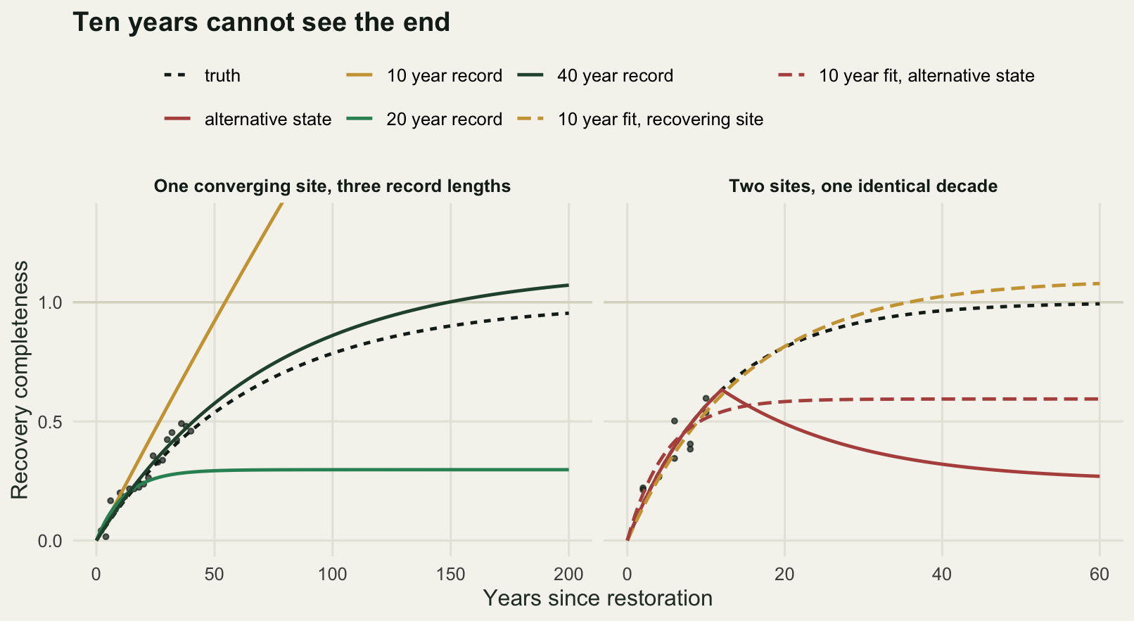
Where to go next
The practical version of all four measurements is a short list for a monitoring plan: report more than one metric and give the spread between them, say which reference you divided by and when it was measured, avoid reading a chronosequence as a time series unless you can show that site quality is only weakly correlated with site age, and refuse to extrapolate an asymptote from a record shorter than about two fifths of the recovery time you are extrapolating. The last one is the expensive one, because it means the answer to “when will this be recovered” is often that nobody can yet say.
If your restoration is a species rather than a habitat, the same arithmetic reappears with a different denominator, and Reintroduction release strategies works through the version where the trajectory is a population size and the reference is a target population.
References
Ruiz-Jaen MC, Aide TM 2005 Restoration Ecology 13(3):569-577 (10.1111/j.1526-100X.2005.00072.x)
Jones HP, Schmitz OJ 2009 PLoS ONE 4(5):e5653 (10.1371/journal.pone.0005653)
Matthews JW, Spyreas G 2010 Journal of Applied Ecology 47(5):1128-1136 (10.1111/j.1365-2664.2010.01862.x)
Walker LR, Wardle DA, Bardgett RD, Clarkson BD 2010 Journal of Ecology 98(4):725-736 (10.1111/j.1365-2745.2010.01664.x)