Priority effects and alternative stable states

Priority effects in R: how strong mutual competition creates two alternative stable states, so the winner is set by arrival order, not competitive rank.

Two species compete for the same space, one arrives a little ahead of the other, and it wins, permanently, even though the two are evenly matched. Run it again with the late arriver first and the outcome flips. Nothing about the species changed; only the order of arrival did. This is a priority effect, and when it is strong enough it means a community has more than one stable configuration it can settle into. Which one you get is a matter of history, not of who is the better competitor.

When competition inverts the usual rule

The Lotka-Volterra competition model has a well-known set of outcomes, and the interesting one is the least discussed. Each species limits itself through its own density and limits its competitor through cross-competition. When a species limits itself more than it limits the other, coexistence follows; that is the stable, familiar case. But when each species limits the other more than itself, the model inverts: whichever species gets ahead suppresses its rival faster than it suppresses itself, so its lead compounds until the rival is gone. Set the cross-competition coefficients above one, so each species is its competitor’s worst enemy, and integrate from two starting points that differ only in who leads.

r1 <- r2 <- 0.5; K1 <- K2 <- 100; a12 <- a21 <- 1.5   # each hurts the other more than itself
step <- function(N, dt = 0.1) {
  dN1 <- r1*N[1]*(1 - (N[1] + a12*N[2])/K1); dN2 <- r2*N[2]*(1 - (N[2] + a21*N[1])/K2)
  pmax(N + c(dN1, dN2)*dt, 0)
}
run <- function(N) { for (t in 1:2000) N <- step(N); round(N) }
rbind(species1_ahead = run(c(60, 40)), species2_ahead = run(c(40, 60)))

               [,1] [,2]
species1_ahead  100    0
species2_ahead    0  100

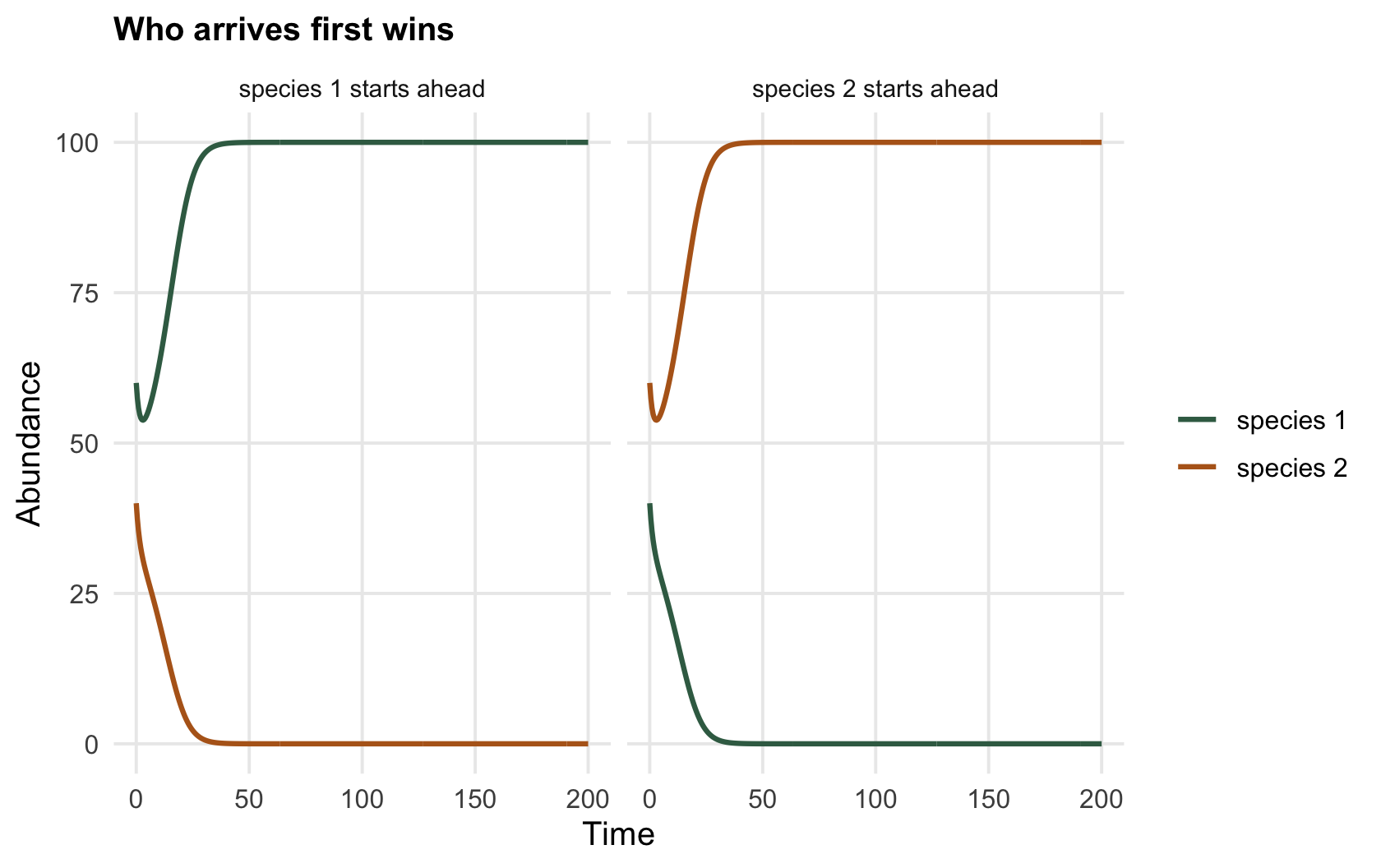
The two runs start as mirror images, 60 against 40 and the reverse, and they end at opposite corners: the first at (100, 0), species 1 alone, the second at (0, 100), species 2 alone. Same species, same competitive strengths, opposite winners. The system has two stable states, monoculture of one or monoculture of the other, and the initial lead decides which basin the community falls into.

d <- rbind(cbind(lv(60, 40), case = "species 1 starts ahead"),
           cbind(lv(40, 60), case = "species 2 starts ahead"))
dl <- reshape(d, varying = c("N1", "N2"), v.names = "N", timevar = "sp", direction = "long")
ggplot(dl, aes(t, N, colour = factor(sp))) +
  geom_line(linewidth = 0.9) + facet_wrap(~case) +
  scale_colour_manual(values = c("1" = col_1, "2" = col_2), labels = c("species 1", "species 2")) +
  labs(x = "Time", y = "Abundance", colour = NULL,
       title = "Who arrives first wins") +
  theme(strip.text = element_text(size = 9))

Figure 1: Two competition runs that differ only in which species starts slightly ahead. Each ends with a different species holding the whole site: the outcome is set by initial conditions, not by the species.

The geometry of two stable states

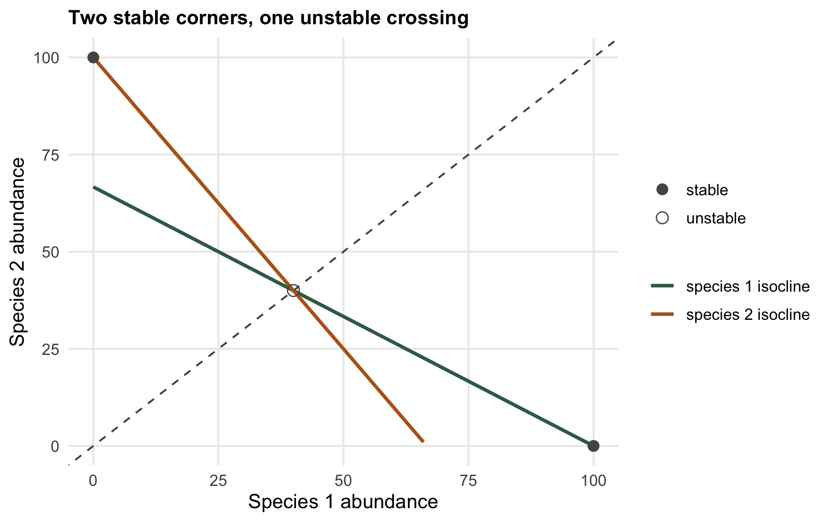
The reason there are two stable states is visible in the zero-growth isoclines, the lines in the abundance plane along which each species stops changing. Species 1 holds steady where its own density plus the pressure from species 2 fills the site; species 2 has its own such line. When cross-competition is strong these two lines cross, and the crossing point is an unstable equilibrium: a knife-edge the community can sit on only if perfectly balanced, and rolls off at the slightest nudge.

N1 <- seq(0, 100, 1)
iso <- rbind(data.frame(N1 = N1, N2 = (K1 - N1)/a12, sp = "species 1 isocline"),
             data.frame(N1 = N1, N2 = K2 - a21*N1,   sp = "species 2 isocline"))
iso <- iso[iso$N2 >= 0 & iso$N2 <= 100, ]
eq <- data.frame(N1 = c(100, 0, Nstar), N2 = c(0, 100, Nstar),
                 kind = c("stable", "stable", "unstable"))
ggplot(iso, aes(N1, N2, colour = sp)) +
  geom_abline(slope = 1, intercept = 0, colour = col_ref, linetype = "dashed") +
  geom_line(linewidth = 1) +
  geom_point(data = eq, aes(N1, N2, shape = kind), colour = col_ref, size = 3, inherit.aes = FALSE) +
  scale_shape_manual(values = c(stable = 16, unstable = 1)) +
  scale_colour_manual(values = c("species 1 isocline" = col_1, "species 2 isocline" = col_2)) +
  labs(x = "Species 1 abundance", y = "Species 2 abundance", colour = NULL, shape = NULL,
       title = "Two stable corners, one unstable crossing")

Figure 2: Zero-growth isoclines for the two species. They cross at an unstable interior point (the critical balance); the two stable states are the corners where one species holds the whole site. The dashed diagonal is the boundary between the two basins.

The unstable crossing sits at 40 of each species, and the two stable states are the corners. A community that starts on one side of the dividing line runs to one corner; start it on the other side and it runs to the other. That dividing line, the basin boundary, is what separates the two histories a community can have.

Why this matters for real communities

Priority effects turn ecology from a story about which species is best into a story about what happened first, and that has consequences a competition ranking cannot capture. Restoration can fail or succeed on the order of planting; an invader that would lose to a resident at equal densities can hold ground once it is established first; the same patch of habitat, under identical conditions, can support different communities depending on its assembly history. The catch is that alternative stable states are genuinely hard to demonstrate in the field, because a community sitting in one state looks much like a community that simply has no alternative, and telling them apart takes the perturbation and hysteresis tests of the checking post rather than a snapshot. The mechanism is real and important; the evidence for it is where the care is needed.

Related tutorials

• Basins of attraction
• Hysteresis and tipping points
• Checking for alternative stable states
• Annual plant competition models

References

• Lewontin RC 1969. Brookhaven Symposia in Biology 22:13-24.
• Fukami T 2015. Annual Review of Ecology, Evolution, and Systematics 46:1-23 (10.1146/annurev-ecolsys-110411-160340).