library(ggplot2)

theme_te <- theme_minimal(base_size = 12) +
  theme(panel.grid.minor = element_blank(),
        plot.background = element_rect(fill = "#f5f4ee", colour = NA),
        panel.background = element_rect(fill = "#f5f4ee", colour = NA))

## the generating (true) coefficients we will try to recover
lamA <- 45; aAA <- 0.10; aAB <- 0.03   # focal A: intra 0.10, inter 0.03
lamB <- 30; aBB <- 0.06; aBA <- 0.06 # focal B coefficients, carried into the next postFitting annual plant competition models
R
competition
coexistence
population ecology
ecology tutorial
Fit Beverton-Holt competition coefficients to annual plant fecundity data in R, and see why the experimental design decides which coefficients you can estimate.
Corrected 30 September 2026: the post called the additive design’s interspecific coefficient well estimated; it now says that estimate, from a small slice of the data, is imprecise.
Coexistence theory rests on a small set of numbers: how fast a plant’s seed output falls as its neighbours crowd in, and whether a conspecific neighbour crowds it harder than a heterospecific one. Those numbers are the competition coefficients, and everything downstream (niche differences, fitness differences, who wins) is computed from them. This post fits them from scratch. The main lesson is not the fitting, which is a two-line nls call, but the design: the experiment you run decides which coefficients you can recover, and the most common design cannot give you the one you need most.
The model
Write the per-capita seed production of a focal plant of species A as a declining function of the number of competing neighbours. The Beverton-Holt form is the standard choice for annual plants:
\[F_A = \frac{\lambda_A}{1 + \alpha_{AA} D_A + \alpha_{AB} D_B}\]
Here \(\lambda_A\) is the seed output with no neighbours, \(D_A\) and \(D_B\) are the densities of conspecific and heterospecific competitors, and the two competition coefficients \(\alpha_{AA}\) and \(\alpha_{AB}\) set how fast fecundity declines with each kind of neighbour. Per-capita output starts at \(\lambda_A\) and falls hyperbolically: one more conspecific costs a lot when the plant is uncrowded and little once it is already surrounded.
The two coefficients answer different questions. \(\alpha_{AA}\) is intraspecific: how much a plant of A suppresses another plant of A. \(\alpha_{AB}\) is interspecific: how much a plant of B suppresses a plant of A. Coexistence theory needs both, because coexistence turns on whether a species limits itself more than it limits its competitor. A design that measures only one of them cannot answer the coexistence question, however clean the data.
Setup
A response-surface experiment
A response-surface design grows focal plants across a grid of conspecific and heterospecific densities, independently varied, and records seed set for each plant. The independence is the point: because both densities move, the fit can tell apart the two coefficients. We simulate one for focal species A, with realistic scatter in seed counts (a negative binomial captures the overdispersion of real seed-set data).
set.seed(101)
gridpts <- c(0, 2, 4, 8, 16, 32)
d <- expand.grid(DA = gridpts, DB = gridpts)
d <- d[rep(seq_len(nrow(d)), each = 6), ]           # 6 focal plants per cell
mu <- lamA / (1 + aAA * d$DA + aAB * d$DB)          # expected seeds per focal plant
d$seeds <- rnbinom(nrow(d), mu = mu, size = 10)      # overdispersed counts
n_plants <- nrow(d)
That is 216 focal plants across 36 density combinations. Fitting the Beverton-Holt model is a direct nonlinear least squares call: no linearisation, no logging of the response.
fit_A <- nls(seeds ~ lam / (1 + aii * DA + aij * DB), data = d,
             start = list(lam = 40, aii = 0.05, aij = 0.05))
cf <- coef(fit_A)
ci <- suppressMessages(confint(fit_A, "aii"))
Code behind this output; later chunks use it, so run it first
lamA_hat <- unname(cf["lam"]); aAA_hat <- unname(cf["aii"]); aAB_hat <- unname(cf["aij"])The fit recovers the generating values: \(\lambda_A\) = 46.2 (true 45), \(\alpha_{AA}\) = 0.110 (true 0.10), \(\alpha_{AB}\) = 0.025 (true 0.03), with a 95% interval on the intraspecific coefficient of [0.083, 0.143].
xx <- seq(0, 32, length.out = 100)
pred <- rbind(
  data.frame(D = xx, seeds = lamA_hat / (1 + aAA_hat * xx), neighbour = "conspecific (A)"),
  data.frame(D = xx, seeds = lamA_hat / (1 + aAB_hat * xx), neighbour = "heterospecific (B)"))
obs <- rbind(
  data.frame(D = d$DA[d$DB == 0], seeds = d$seeds[d$DB == 0], neighbour = "conspecific (A)"),
  data.frame(D = d$DB[d$DA == 0], seeds = d$seeds[d$DA == 0], neighbour = "heterospecific (B)"))
ggplot(pred, aes(D, seeds, colour = neighbour)) +
  geom_point(data = obs, alpha = 0.4, size = 1.4) +
  geom_line(linewidth = 1) +
  scale_colour_manual(values = c("conspecific (A)" = "#275139",
                                 "heterospecific (B)" = "#b5534e")) +
  labs(x = "neighbour density (plants per plot)",
       y = "seeds per focal plant", colour = NULL) +
  theme_te + theme(legend.position = "top")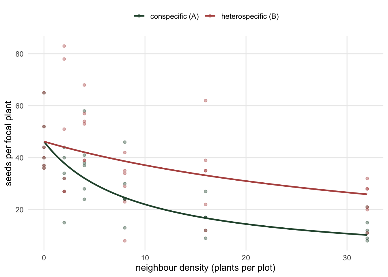
The conspecific curve drops faster: a plant of A is hurt more by another A than by a B. That gap between \(\alpha_{AA}\) and \(\alpha_{AB}\) is the seed of a niche difference, and it is exactly what an average-density analysis destroys. Lumping all neighbours into one “total density” predictor forces \(\alpha_{AA}\) = \(\alpha_{AB}\) by construction, discarding the asymmetry that decides coexistence.
Why the additive design cannot help you
The response-surface grid is more work than the design most competition experiments actually use. The common alternative is additive: hold the focal density fixed (often at zero, so a lone focal plant grows against a gradient of the other species) and vary only the competitor. It is cheaper, and it estimates the interspecific effect. It also cannot estimate the intraspecific coefficient, and no amount of replication fixes that.
Take the slice of our data with no conspecific neighbours and try to fit all three parameters:
add <- d[d$DA == 0, ]
result <- tryCatch(
  nls(seeds ~ lam / (1 + aii * DA + aij * DB), data = add,
      start = list(lam = 40, aii = 0.05, aij = 0.05)),
  error = function(e) conditionMessage(e))
n_add <- nrow(add)
result
[1] "singular gradient matrix at initial parameter estimates"The fit fails with a singular gradient: with conspecific density fixed at zero, the data contain no information about how conspecifics compete, so \(\alpha_{AA}\) is not identified. This is not a starting-value problem. Dropping the unidentified term does fit, and estimates \(\lambda_A\) and \(\alpha_{AB}\) from the same 36 plants:
fit_add <- nls(seeds ~ lam / (1 + aij * DB), data = add,
               start = list(lam = 40, aij = 0.05))
round(coef(fit_add), 3)
lam aij
49.742 0.036 So the additive design gives you a real interspecific coefficient, though an imprecise one from only 36 plants, and nothing at all about self-limitation. The reason is worth seeing directly. If we fix the intraspecific coefficient at a grid of values and refit the rest, the residual sum of squares tells us how much the data care about that coefficient.
prof_rss <- function(dat, grid) sapply(grid, function(a) {
  f <- try(nls(seeds ~ lam / (1 + a * DA + aij * DB), data = dat,
               start = list(lam = 40, aij = 0.05)), silent = TRUE)
  if (inherits(f, "try-error")) NA_real_ else sum(residuals(f)^2)
})
agrid <- seq(0, 0.30, by = 0.01)
prof <- rbind(
  data.frame(aii = agrid, rss = prof_rss(d, agrid),   design = "response surface"),
  data.frame(aii = agrid, rss = prof_rss(add, agrid), design = "additive (conspecific absent)"))
prof$rel <- ave(prof$rss, prof$design, FUN = function(z) z / min(z, na.rm = TRUE))
ggplot(prof, aes(aii, rel, colour = design)) +
  geom_line(linewidth = 1) +
  scale_colour_manual(values = c("response surface" = "#275139",
                                 "additive (conspecific absent)" = "#b5534e")) +
  labs(x = expression("intraspecific coefficient " * alpha[AA]),
       y = "residual sum of squares (relative to minimum)", colour = NULL) +
  theme_te + theme(legend.position = "top")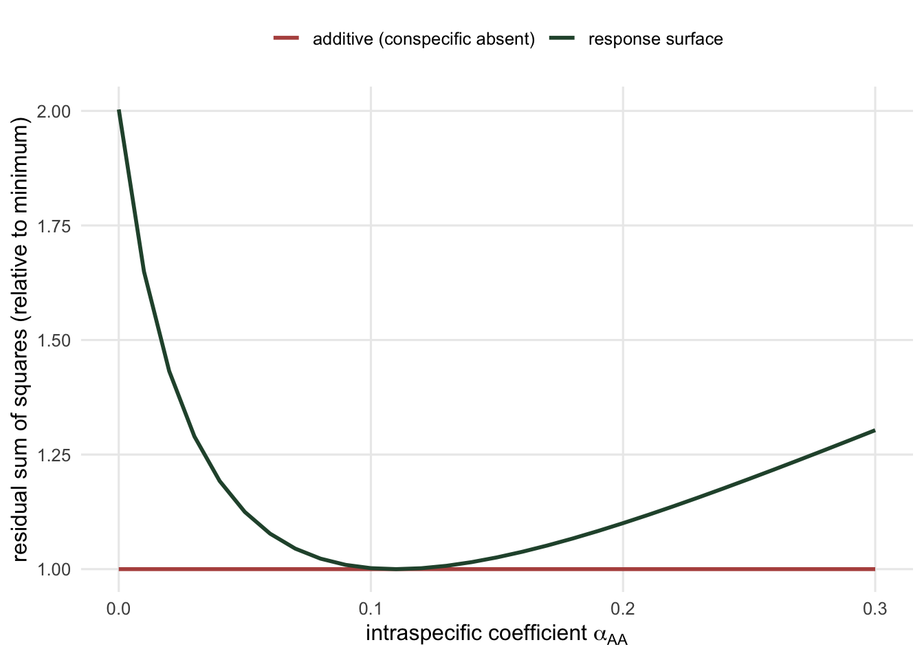
The flat line is the whole problem: under the additive design the intraspecific coefficient is unidentified, and that is the coefficient coexistence theory needs most. The whole question is whether intraspecific competition exceeds interspecific competition, and the additive design measures only the second term. You can run a beautiful additive experiment, publish tidy interspecific effects, and be unable to say anything about coexistence, because the comparison you need was never in the design.
The response-surface design is not a refinement for the fastidious; it is the minimum that identifies the coefficients coexistence theory is built from. In the next post we take a full set of fitted coefficients (both focal species) and turn them into niche and fitness differences, and see why the stronger competitor does not always win.
References
Hart SP, Freckleton RP, Levine JM 2018. Journal of Ecology 106(5):1902-1909 (10.1111/1365-2745.12954).
Godoy O, Kraft NJB, Levine JM 2014. Ecology Letters 17(7):836-844 (10.1111/ele.12289).
Levine JM, HilleRisLambers J 2009. Nature 461(7261):254-257 (10.1038/nature08251).