set.seed(4221)
a_true <- 1.2
h_true <- 0.045
dens   <- rep(c(2, 4, 8, 16, 32, 50, 75, 100), each = 4)
mu     <- a_true * dens / (1 + a_true * h_true * dens)   # expected number eaten
Ne     <- rpois(length(dens), mu)
d <- data.frame(N = dens, Ne = Ne)Nonlinear regression in R with nls
R
nonlinear regression
functional response
ecology tutorial
Fitting nonlinear models in R with nls: why linearising a functional response biases attack rate and handling time, and how direct least squares recovers them.
Many ecological relationships are nonlinear in the parameters: a functional response, a growth curve, a decay curve, a dose response. The quickest way to fit them with a tool you already know is to transform both sides until the model looks linear, then reach for lm. That shortcut is tempting and, for parameter estimation, usually wrong. Transforming to a straight line moves the error onto a scale where it is no longer even roughly constant or symmetric, and the least squares fit on that scale answers a different question than the one you asked.
This post uses the Holling type II functional response as the running example, because its linearisation is a textbook case. The lesson is general: fit the nonlinear model on its own scale with nls, and treat the transformation trick as a way to get starting values, not final estimates.
The model
A type II functional response describes the number of prey a predator eats as prey density rises. The disc equation (Holling 1959) gives the expected number eaten as
\[ N_e = \frac{a\,N}{1 + a\,h\,N}, \]
with two parameters: the attack rate \(a\) (how fast the predator finds prey at low density) and the handling time \(h\) (the time tied up per prey, which sets the plateau \(1/h\) at high density). We simulate a feeding experiment in which a predator is offered a range of prey densities, each replicated, with prey continually replaced so that the disc equation holds exactly. The counts eaten are Poisson around the expected curve.
The naive shortcut: a double reciprocal
Take reciprocals of both sides of the disc equation and it straightens out:
\[ \frac{1}{N_e} = h + \frac{1}{a}\cdot\frac{1}{N}. \]
So a straight line of \(1/N_e\) against \(1/N\) has intercept \(h\) and slope \(1/a\). This is the Lineweaver-Burk plot, borrowed from enzyme kinetics. It is easy, but it has two problems baked in. First, the reciprocal is undefined whenever no prey are eaten, so any trial with a zero count has to be dropped, throwing away exactly the low density information the fit leans on; this particular draw happens to contain no zeros, so here only the second problem bites. Second, taking reciprocals stretches the small counts (the noisy low density trials) across a huge range of \(1/N_e\) and compresses the large counts near zero, so ordinary least squares on this scale is dominated by the least reliable points.
dpos <- d[d$Ne > 0, ]                       # 1/Ne is undefined at Ne = 0
lb   <- lm(I(1 / Ne) ~ I(1 / N), data = dpos)
a_lin <- unname(1 / coef(lb)[2])
h_lin <- unname(coef(lb)[1])
On this dataset the double reciprocal returns an attack rate of 0.931 and a handling time of 0.0607, against the true values of 1.2 and 0.045. The handling time is badly overstated, which drags the implied plateau \(1/h\) down to 16.5 prey when the truth is 22.2.
The direct fit: nls
nls minimises the squared residuals on the original scale, where the Poisson error actually lives, using Gauss-Newton iteration. It needs starting values. Rather than guess, notice that the disc equation is a Michaelis-Menten curve in disguise: writing \(V_m = 1/h\) and \(K = 1/(a h)\) gives \(N_e = V_m N / (K + N)\), and base R ships a self-starting Michaelis-Menten model that finds its own starting values. We fit that, back-transform to \(a\) and \(h\), and use those as the starting point for the disc equation in its native form.
ss  <- nls(Ne ~ SSmicmen(N, Vm, K), data = d)     # self-starting, no guesses
Vm  <- unname(coef(ss)["Vm"]); K <- unname(coef(ss)["K"])
fit <- nls(Ne ~ a * N / (1 + a * h * N), data = d,
           start = list(a = Vm / K, h = 1 / Vm))
a_hat <- unname(coef(fit)["a"]); h_hat <- unname(coef(fit)["h"])
The direct fit gives an attack rate of 1.246 and a handling time of 0.0419, both close to the truth, and its plateau \(1/h\) of 23.9 sits right where the data level off. The two fitted curves tell the story: the direct fit tracks the plateau, while the linearised curve bends down far too early because its handling time is inflated.
library(ggplot2)
theme_te <- function(base_size = 12) {
  theme_minimal(base_size = base_size) +
    theme(plot.background  = element_rect(fill = "#f5f4ee", colour = NA),
          panel.background = element_rect(fill = "#f5f4ee", colour = NA),
          panel.grid.minor = element_blank(),
          panel.grid.major = element_line(colour = "#dad9ca", linewidth = 0.3),
          axis.title = element_text(colour = "#2c3a31"),
          axis.text  = element_text(colour = "#46604a"),
          plot.subtitle = element_text(colour = "#5d6b61"),
          legend.position = "top",
          legend.title = element_blank(),
          legend.text  = element_text(colour = "#46604a"))
}
grid <- data.frame(N = seq(1, 105, length.out = 300))
grid$nls <- a_hat * grid$N / (1 + a_hat * h_hat * grid$N)
grid$lin <- a_lin * grid$N / (1 + a_lin * h_lin * grid$N)
ggplot(d, aes(N, Ne)) +
  geom_point(colour = "#16241d", alpha = 0.7, size = 1.9) +
  geom_line(data = grid, aes(N, nls, colour = "direct nls"), linewidth = 1) +
  geom_line(data = grid, aes(N, lin, colour = "double reciprocal"),
            linewidth = 1, linetype = "21") +
  scale_colour_manual(values = c("direct nls" = "#275139",
                                 "double reciprocal" = "#b5534e")) +
  labs(x = "prey density N", y = "prey eaten", subtitle =
       "Same data, two fitting methods") +
  theme_te()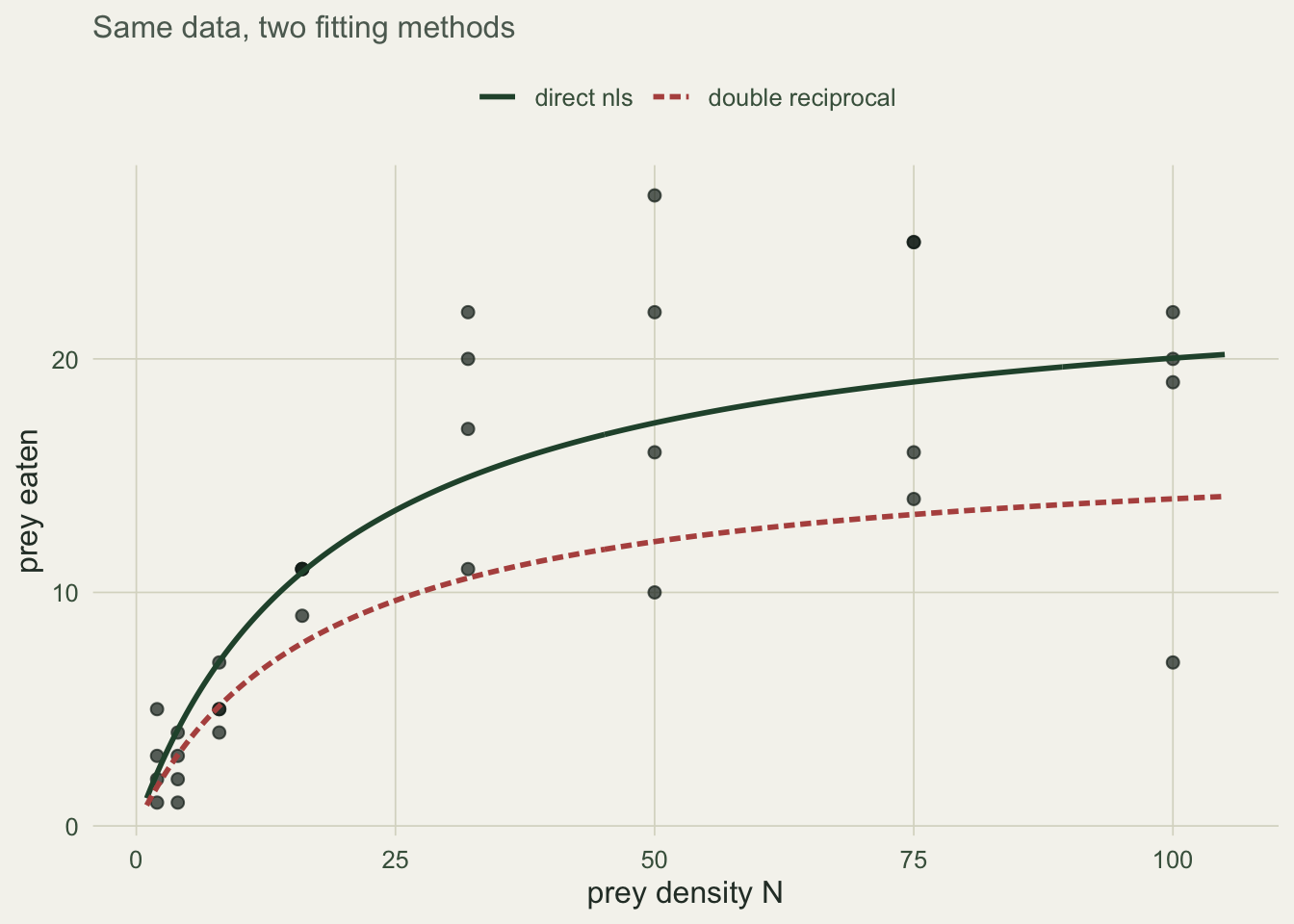
Why the linearisation is biased, not just noisy
One dataset could be a fluke, so we repeat the whole experiment many times and refit both ways. This separates bias (does the method land on the truth on average?) from efficiency (how much does it scatter?).
set.seed(20260810)
B  <- 2000
mc <- matrix(NA_real_, B, 2, dimnames = list(NULL, c("a_nls", "a_lin")))
for (b in seq_len(B)) {
  Neb <- rpois(length(dens), mu)
  db  <- data.frame(N = dens, Ne = Neb)
  fb  <- try(nls(Ne ~ a * N / (1 + a * h * N), data = db,
                 start = list(a = 1, h = 0.04)), silent = TRUE)
  if (!inherits(fb, "try-error")) mc[b, 1] <- coef(fb)["a"]
  dp  <- db[db$Ne > 0, ]
  mc[b, 2] <- 1 / coef(lm(I(1 / Ne) ~ I(1 / N), data = dp))[2]
}
mc     <- mc[complete.cases(mc), ]
bias_nls <- mean(mc[, 1]) / a_true - 1
bias_lin <- mean(mc[, 2]) / a_true - 1
sd_nls   <- sd(mc[, 1]); sd_lin <- sd(mc[, 2])
Across 2000 simulated experiments the direct fit is essentially unbiased for the attack rate (mean 1.222, a relative bias of 1.8 per cent), while the double reciprocal underestimates it by 12.1 per cent (mean 1.055). The linearised estimator is also noisier: its standard deviation is 0.332 against 0.251 for nls. So the transformation costs on both fronts at once, systematic bias and lower precision, because it is fitting the wrong error structure.
mcl <- data.frame(
  a = c(mc[, 1], mc[, 2]),
  method = rep(c("direct nls", "double reciprocal"), each = nrow(mc)))
ggplot(mcl, aes(a, fill = method, colour = method)) +
  geom_density(alpha = 0.35, linewidth = 0.6) +
  geom_vline(xintercept = a_true, colour = "#16241d", linetype = "31") +
  scale_fill_manual(values = c("direct nls" = "#275139",
                               "double reciprocal" = "#b5534e")) +
  scale_colour_manual(values = c("direct nls" = "#275139",
                                 "double reciprocal" = "#b5534e")) +
  coord_cartesian(xlim = c(0.4, 2.4)) +
  labs(x = "estimated attack rate", y = "density", subtitle =
       "Dashed line is the true attack rate") +
  theme_te()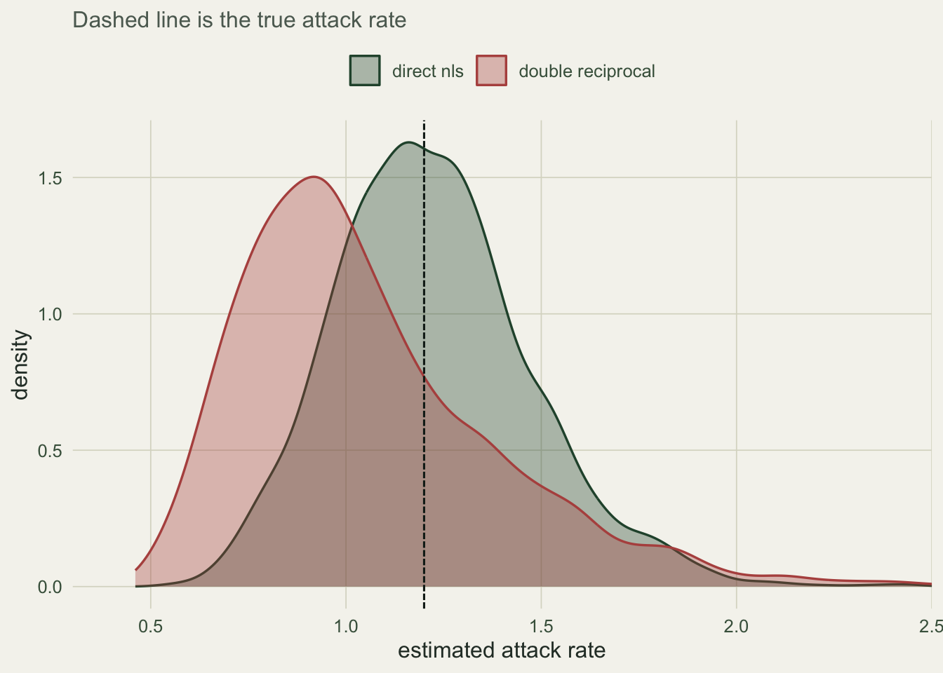
Confidence intervals: profile, not Wald
The summary of an nls fit reports a standard error for each parameter, and it is tempting to build a symmetric interval as estimate plus or minus twice that. For nonlinear parameters the sampling distribution is often skewed, so a symmetric interval misplaces both ends. The confint method profiles the likelihood instead, tracing how the fit degrades as each parameter is held away from its best value.
se_a  <- summary(fit)$coefficients["a", "Std. Error"]
wald  <- a_hat + c(-1, 1) * 1.96 * se_a
prof  <- suppressMessages(confint(fit, "a"))
Here the Wald interval for the attack rate is 0.57 to 1.93, while the profile interval is 0.76 to 2.11. The profile interval is not symmetric about the estimate: its upper arm (0.87) is longer than its lower arm (0.49), because a high attack rate is harder to rule out than a low one. Prefer the profile interval; the checking post in this series returns to why the Wald version can be over-optimistic.
The honest limit
nls gives you back what the double reciprocal throws away, but it is not a free lunch. It needs starting values, and for awkward models a poor start can send it to a false solution or no solution at all; that is the subject of a later post in this series. More importantly, the whole exercise assumes the disc equation is the right shape. If prey deplete during the trial (they are eaten and not replaced), the disc equation no longer holds and you need the Rogers random-predator equation instead, which has no closed form and is fitted through the Lambert W function. And a type II shape is itself a choice: a type III response, where attack rate rises with density, can look similar over a narrow range. The fit is only as trustworthy as the functional form you assumed, and no amount of clever estimation tests that form for you. The next post fits growth curves the same way, and shows how strongly the parameters can trade off.
Where to go next
The companion posts fit growth curves with nls, work through starting values and identifiability, and check a nonlinear fit properly. For the diagnostics behind lm residuals that carry over here, see the GLM diagnostics post; for the general idea of simulating to separate bias from noise, see the power analysis post.
References
- Holling 1959 Canadian Entomologist 91(7):385-398 (10.4039/Ent91385-7)
- Rogers 1972 Journal of Animal Ecology 41(2):369-383 (10.2307/3474)
- Trexler, McCulloch and Travis 1988 Oecologia 76(2):206-214 (10.1007/BF00379954)
- Juliano 2001 in Scheiner and Gurevitch (eds), Design and Analysis of Ecological Experiments, 2nd ed, Oxford University Press (ISBN 978-0-19-513187-1)
- Bates and Watts 1988, Nonlinear Regression Analysis and Its Applications, Wiley (ISBN 978-0-471-81643-0)
- Bolker 2008, Ecological Models and Data in R, Princeton University Press (ISBN 978-0-691-12522-0)
- Motulsky and Ransnas 1987 FASEB Journal 1(5):365-374 (10.1096/fasebj.1.5.3315805)