set.seed(4196)
tt <- rep(seq(0, 12, by = 0.5), each = 3)
A1 <- 5; r1 <- 1.2; A2 <- 3; r2 <- 0.18; s <- 0.15
y  <- A1 * exp(-r1 * tt) + A2 * exp(-r2 * tt) + rnorm(length(tt), 0, s)
d <- data.frame(t = tt, y = y)Starting values and identifiability in nls
R
nonlinear regression
model fitting
ecology tutorial
Why nls fails to converge, and why it converges to a parameter that was never identifiable: starting values, self-start models and flat likelihoods in R.
Corrected 27 September 2026: the profile figure drew a few constrained refits that had not converged, which made the close-rates curve zig-zag at its left end; those points are now left out, as the code comment always said.
nls can fail in two very different ways, and telling them apart matters. Sometimes it stops before it starts, with an error and no fit. Sometimes it returns a tidy set of estimates, one of which is meaningless because the data never contained the information to pin it down. The first is a starting-value problem and is fixable. The second is an identifiability problem and is not fixable by any amount of better optimisation. This post works through both using a two-pool decay curve, the kind you meet in decomposition, drug clearance, or a die-off with a fast and a slow phase.
A model that will not start
A biexponential sums a fast and a slow decay,
\[ y(t) = A_1 e^{-r_1 t} + A_2 e^{-r_2 t}, \]
with two amplitudes and two rate constants. We simulate a clean example where the two rates are well separated.
A first instinct is to hand nls some round-number starting values and let it run. With this model that fails immediately.
naive <- try(nls(y ~ a1 * exp(-b1 * t) + a2 * exp(-b2 * t), data = d,
                 start = list(a1 = 1, b1 = 1, a2 = 1, b2 = 1)), silent = TRUE)
msg <- trimws(conditionMessage(attr(naive, "condition")))
nls stops with the error: singular gradient matrix at initial parameter estimates. That message means the four columns of the design derivative are nearly linearly dependent at the starting point, so the Gauss-Newton step cannot be computed. It is not saying the model is wrong; it is saying the starting values are too poor for the first step.
Self-starting solves it
Base R ships self-starting model builders that find their own starting values from the shape of the data. SSbiexp is exactly the biexponential, parameterised with log rate constants so the rates stay positive. It converges without any guesses.
ss  <- nls(y ~ SSbiexp(t, A1, lrc1, A2, lrc2), data = d)
cs  <- coef(ss)
fit <- nls(y ~ a1 * exp(-b1 * t) + a2 * exp(-b2 * t), data = d,
           start = list(a1 = unname(cs["A1"]), b1 = unname(exp(cs["lrc1"])),
                        a2 = unname(cs["A2"]), b2 = unname(exp(cs["lrc2"]))))
co  <- coef(fit)
It recovers a fast pool of amplitude 5.17 decaying at 1.208 and a slow pool of amplitude 2.86 decaying at 0.168, against the true amplitudes of 5 and 3 and rates of 1.2 and 0.18. Splitting the fitted curve into its two pools shows what the model is doing: a steep early drop from the fast pool sitting on a long tail from the slow one.
library(ggplot2)
theme_te <- function(base_size = 12) {
  theme_minimal(base_size = base_size) +
    theme(plot.background  = element_rect(fill = "#f5f4ee", colour = NA),
          panel.background = element_rect(fill = "#f5f4ee", colour = NA),
          panel.grid.minor = element_blank(),
          panel.grid.major = element_line(colour = "#dad9ca", linewidth = 0.3),
          axis.title = element_text(colour = "#2c3a31"),
          axis.text  = element_text(colour = "#46604a"),
          plot.subtitle = element_text(colour = "#5d6b61"),
          legend.position = "top", legend.title = element_blank(),
          legend.text = element_text(colour = "#46604a"))
}
gg <- data.frame(t = seq(0, 12, length.out = 300))
gg$fit  <- predict(fit, gg)
gg$fast <- co["a1"] * exp(-co["b1"] * gg$t)
gg$slow <- co["a2"] * exp(-co["b2"] * gg$t)
p_decomp <- ggplot(d, aes(t, y)) +
  geom_point(colour = "#16241d", alpha = 0.55, size = 1.5) +
  geom_line(data = gg, aes(t, fit),  colour = "#275139", linewidth = 1) +
  geom_line(data = gg, aes(t, fast), colour = "#b5534e", linewidth = 0.8, linetype = "21") +
  geom_line(data = gg, aes(t, slow), colour = "#cda23f", linewidth = 0.8, linetype = "41") +
  labs(x = "time", y = "response", subtitle =
       "Green: fit. Red: fast pool. Gold: slow pool") +
  theme_te()
p_decomp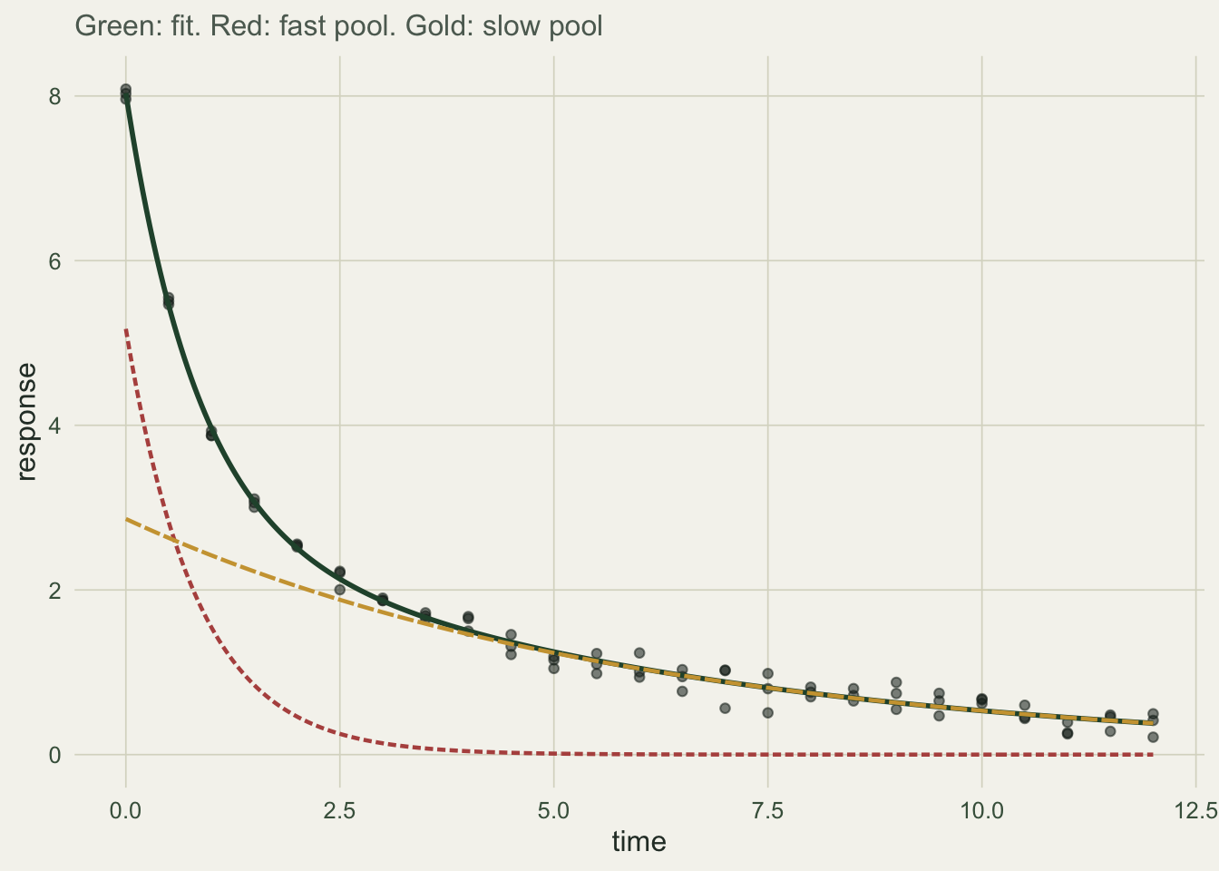
Reparameterise to make the fit easier
Even when a fit converges, the parameters can be needlessly correlated, which slows convergence and makes profiling fragile. A single decay makes the point cleanly. Fitting \(y = a\,e^{-b t}\) with time starting at zero, the amplitude and the rate are correlated because the amplitude is the height at \(t = 0\), far from where the rate is actually informed.
set.seed(4296)
tr <- rep(seq(0, 10, by = 0.5), each = 4)
yr <- 4 * exp(-0.35 * tr) + rnorm(length(tr), 0, 0.12)
dr <- data.frame(t = tr, y = yr)
f_raw <- nls(y ~ a * exp(-b * t),          data = dr, start = list(a = 3, b = 0.3))
f_ctr <- nls(y ~ a * exp(-b * (t - 1.2)),  data = dr, start = list(a = 1, b = 0.3))
c_raw <- cov2cor(vcov(f_raw))["a", "b"]
c_ctr <- cov2cor(vcov(f_ctr))["a", "b"]
Shifting the time origin to a point inside the decay, here \(t = 1.2\), drops the amplitude-rate correlation from 0.65 to 0.01, while the rate estimate is unchanged at 0.342. The fit is identical; the parameters are just cleaner to estimate. This is the general idea behind Ratkowsky’s close-to-linear parameterisations: rewrite the model so the parameters are close to orthogonal and their profiles close to parabolic.
The unfixable case: parameters that are not identified
Now change one thing about the two-pool model: make the two rates similar rather than well separated. Everything about the fitting code stays the same.
set.seed(4396)
yc  <- A1 * exp(-0.45 * tt) + A2 * exp(-0.30 * tt) + rnorm(length(tt), 0, s)
dc  <- data.frame(t = tt, y = yc)
ssc <- nls(y ~ SSbiexp(t, A1, lrc1, A2, lrc2), data = dc,
           control = nls.control(maxiter = 500, warnOnly = TRUE))
fitc <- nls(y ~ a1 * exp(-b1 * t) + a2 * exp(-b2 * t), data = dc,
            start = list(a1 = unname(coef(ssc)["A1"]), b1 = unname(exp(coef(ssc)["lrc1"])),
                         a2 = unname(coef(ssc)["A2"]), b2 = unname(exp(coef(ssc)["lrc2"]))),
            control = nls.control(maxiter = 500, warnOnly = TRUE))
corr_aa <- cov2cor(vcov(fitc))["a1", "a2"]
se_b1   <- summary(fitc)$coefficients["b1", "Std. Error"]
The fit returns numbers, but they are not to be trusted. The two amplitudes are correlated at -0.997, almost perfectly opposed: the fit can trade amplitude from one pool to the other with barely any change in fit. The fast rate is estimated at 0.92 when the truth is 0.45, with a standard error of 0.73. When two decay rates are close, their sum looks like a single curved decay.
The clearest diagnostic is to profile a rate: fix it at a grid of values, refit everything else, and watch the residual sum of squares. A well-determined parameter gives a valley; an unidentified one gives a flat floor.
prof_b1 <- function(dat, grid, st) sapply(grid, function(v) {
  fr <- try(nls(y ~ a1 * exp(-v * t) + a2 * exp(-b2 * t), data = dat, start = st,
                control = nls.control(maxiter = 200, warnOnly = TRUE)), silent = TRUE)
  if (inherits(fr, "try-error") || !fr$convInfo$isConv) NA_real_ else sum(resid(fr)^2)
})
gsep <- seq(0.5, 2.2, length.out = 60)
gcls <- seq(0.30, 1.6, length.out = 60)
rss_sep <- prof_b1(d,  gsep, list(a1 = 5, a2 = 3, b2 = 0.18))
rss_cls <- prof_b1(dc, gcls, list(a1 = 5, a2 = 3, b2 = 0.30))
rss_sep <- rss_sep - min(rss_sep, na.rm = TRUE)
rss_cls <- rss_cls - min(rss_cls, na.rm = TRUE)
pf <- rbind(
data.frame(b1 = gsep, rss = rss_sep, case = "rates well separated"),
data.frame(b1 = gcls, rss = rss_cls, case = "rates close together"))
# prof_b1() records NA where the constrained refit does not converge, which happens at the
# extreme end of the close-rates grid: there is no profile value there to draw
pf <- pf[!is.na(pf$rss), ]
ggplot(pf, aes(b1, rss, colour = case)) +
geom_line(linewidth = 1) +
coord_cartesian(ylim = c(0, 6)) +
scale_colour_manual(values = c("rates well separated" = "#275139",
"rates close together" = "#b5534e")) +
labs(x = "fixed fast rate", y = "residual sum of squares above minimum",
subtitle = "A flat floor means the rate is not identified") +
theme_te()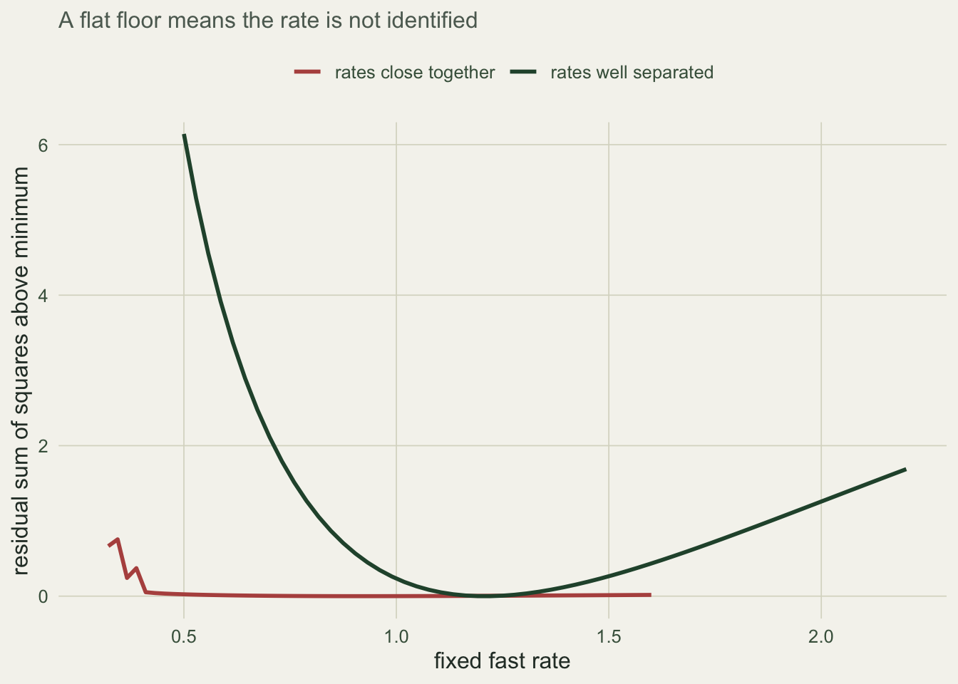
The separated case has a sharp minimum near the true rate, so the data pin it down. The close case is almost flat: a fast rate of 0.5 and one of 1.5 fit within a whisker of each other. Fitting a single exponential to the close-rate data raises the residual sum of squares only slightly, and by AIC the second pool is barely worth its two extra parameters.
The honest limit
A converged fit is not evidence that its parameters are identified. Identifiability is a joint property of the model and the design, not something the optimiser decides, so when a parameter is not identified no starting-value trick, no reparameterisation, and no alternative algorithm will recover it. The profile tells you which case you are in: a valley means the data speak, a flat floor means they do not. When you meet a flat floor you have two honest options, and neither is to report the number anyway. You can simplify the model to what the data support, here a single pool. Or you can change the design so the components separate, by sampling longer to let the slow pool show, or more precisely to resolve the fast one. The next post takes a fitted, identified model and works through checking it: residuals, the right kind of interval, and what an extrapolated prediction does and does not tell you.
References
- Bates and Watts 1988, Nonlinear Regression Analysis and Its Applications, Wiley (ISBN 978-0-471-81643-0)
- Ratkowsky 1986 Canadian Journal of Fisheries and Aquatic Sciences 43(4):742-747 (10.1139/f86-091)
- Seber and Wild 1989, Nonlinear Regression, Wiley (ISBN 978-0-471-61760-0)
- Bolker 2008, Ecological Models and Data in R, Princeton University Press (ISBN 978-0-691-12522-0)
- Raue et al. 2009 Bioinformatics 25(15):1923-1929 (10.1093/bioinformatics/btp358)