set.seed(4195)
Linf <- 60; k <- 0.25; t0 <- -0.5; sigma <- 3
ages <- rep(1:14, each = 6)
L    <- Linf * (1 - exp(-k * (ages - t0))) + rnorm(length(ages), 0, sigma)
d <- data.frame(t = ages, L = L)Fitting growth curves with nls
R
nonlinear regression
growth
ecology tutorial
Fit a von Bertalanffy growth curve in R with nls: why the Ford-Walford plot is noisier than direct fitting, and why the asymptote needs the ages sampled.
Growth curves are one of the most common nonlinear models in ecology: length or mass against age, levelling off towards an asymptotic size. The von Bertalanffy growth function (von Bertalanffy 1938) is the fisheries standard,
\[ L(t) = L_\infty\bigl(1 - e^{-k(t - t_0)}\bigr), \]
with an asymptotic length \(L_\infty\), a growth coefficient \(k\) that sets how fast the curve approaches it, and \(t_0\), the notional age at length zero. This post fits it with nls, contrasts the old graphical shortcut, and then spends most of its time on the parameter that causes the most trouble: the asymptote, which is an extrapolation whenever your oldest animals have not stopped growing.
Simulated length at age
We simulate a cross-sectional sample: several fish at each integer age, lengths scattered around the true curve.
The old shortcut: the Ford-Walford plot
Before nonlinear fitting was routine, growth parameters were read off a straight line. The Ford-Walford plot (Walford 1946) regresses mean length at age \(t+1\) against mean length at age \(t\). Since \(L_{t+1} = L_\infty(1 - e^{-k}) + e^{-k}L_t\), the slope estimates \(e^{-k}\) and the intercept fixes \(L_\infty\).
am  <- tapply(d$L, d$t, mean)
fw  <- lm(am[-1] ~ am[-length(am)])
k_fw    <- unname(-log(coef(fw)[2]))
Linf_fw <- unname(coef(fw)[1] / (1 - coef(fw)[2]))
It has two weaknesses. It needs equal age spacing, which rules it out for the irregular ages that real otolith or scale readings produce. And it pairs and averages, throwing away the within-age scatter, so even when it is roughly unbiased it is noisier than fitting all the points at once. On this dataset it returns an asymptote of 59.4 and a growth coefficient of 0.277.
The direct fit: nls
nls fits the curve to every fish at once, on the length scale where the error lives. Sensible starting values are easy here: the asymptote is near the largest fish, \(k\) is order a few tenths, and \(t_0\) is near zero.
fit <- nls(L ~ Linf * (1 - exp(-k * (t - t0))), data = d,
           start = list(Linf = max(L), k = 0.3, t0 = 0))
co  <- coef(fit)
The direct fit gives an asymptote of 59.4, a growth coefficient of 0.266, and \(t_0\) of -0.39, against the true 60, 0.25 and -0.5.
library(ggplot2)
theme_te <- function(base_size = 12) {
  theme_minimal(base_size = base_size) +
    theme(plot.background  = element_rect(fill = "#f5f4ee", colour = NA),
          panel.background = element_rect(fill = "#f5f4ee", colour = NA),
          panel.grid.minor = element_blank(),
          panel.grid.major = element_line(colour = "#dad9ca", linewidth = 0.3),
          axis.title = element_text(colour = "#2c3a31"),
          axis.text  = element_text(colour = "#46604a"),
          plot.subtitle = element_text(colour = "#5d6b61"),
          legend.position = "top", legend.title = element_blank(),
          legend.text = element_text(colour = "#46604a"))
}
dy   <- d[d$t <= 6, ]
fity <- nls(L ~ Linf * (1 - exp(-k * (t - t0))), data = dy,
            start = list(Linf = 60, k = 0.25, t0 = 0),
            control = nls.control(warnOnly = TRUE))
gg <- data.frame(t = seq(0, 14, length.out = 200))
gg$full  <- predict(fit,  gg)
gg$young <- predict(fity, gg)
ggplot(d, aes(t, L)) +
  geom_point(aes(colour = ifelse(t <= 6, "age 6 or under", "older")),
             alpha = 0.7, size = 1.8) +
  geom_line(data = gg, aes(t, full),  colour = "#275139", linewidth = 1) +
  geom_line(data = gg, aes(t, young), colour = "#b5534e", linewidth = 1,
            linetype = "21") +
  geom_hline(yintercept = Linf, colour = "#16241d", linetype = "31") +
  scale_colour_manual(values = c("age 6 or under" = "#b5534e",
                                  "older" = "#93a87f")) +
  labs(x = "age (years)", y = "length (cm)", subtitle =
       "Dashed red: fit from young fish only; dark line: true asymptote") +
  theme_te()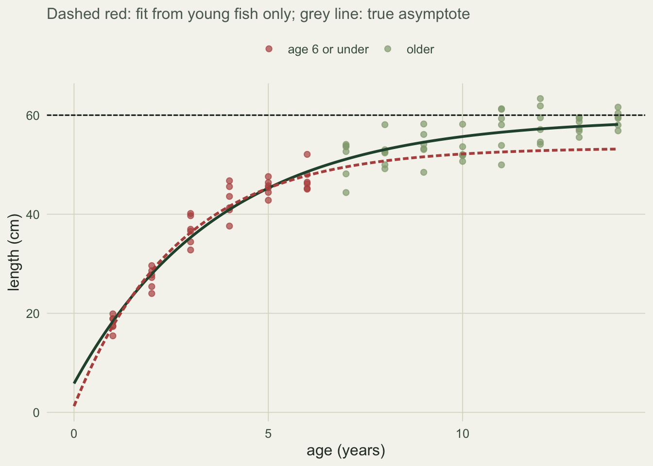
The Ford-Walford plot is noisier, not just old-fashioned
Repeating the sampling many times shows both methods land near the truth on clean data, but the Ford-Walford estimates scatter more, because pairing age means discards information the direct fit keeps.
set.seed(20260811)
B  <- 2000
mc <- matrix(NA_real_, B, 4, dimnames = list(NULL, c("Lnls","knls","Lfw","kfw")))
for (b in seq_len(B)) {
  Lb <- Linf * (1 - exp(-k * (ages - t0))) + rnorm(length(ages), 0, sigma)
  db <- data.frame(t = ages, L = Lb)
  fb <- try(nls(L ~ Linf * (1 - exp(-k * (t - t0))), data = db,
                start = list(Linf = 60, k = 0.25, t0 = 0),
                control = nls.control(warnOnly = TRUE)), silent = TRUE)
  if (!inherits(fb, "try-error") && fb$convInfo$isConv) {
    mc[b, 1] <- coef(fb)["Linf"]; mc[b, 2] <- coef(fb)["k"] }
  amb <- tapply(db$L, db$t, mean)
  sl  <- coef(lm(amb[-1] ~ amb[-length(amb)]))[2]
  if (sl > 0 && sl < 1) { mc[b, 3] <- coef(lm(amb[-1] ~ amb[-length(amb)]))[1] / (1 - sl)
                          mc[b, 4] <- -log(sl) }
}
mc <- mc[complete.cases(mc), ]
eff_L <- sd(mc[, 3]) / sd(mc[, 1]); eff_k <- sd(mc[, 4]) / sd(mc[, 2])
Over 1999 runs the asymptote averages 60.1 for nls and 59.6 for Ford-Walford, both near the true 60, but the Ford-Walford asymptote is 1.25 times as variable and its growth coefficient 1.38 times as variable. Direct fitting keeps that precision and, unlike the graphical method, copes with unequal ages.
Which growth curve?
The von Bertalanffy shape is a choice, not a law. Two other asymptotic forms, the Gompertz and the logistic, fit the same kind of data, so it is worth comparing them rather than assuming one.
fg <- nls(L ~ Linf * exp(-b * exp(-k * t)), data = d,
          start = list(Linf = max(L), b = 2, k = 0.3))
fl <- nls(L ~ Linf / (1 + exp(-k * (t - tm))), data = d,
          start = list(Linf = max(L), k = 0.4, tm = 3))
aic <- c(vonBert = AIC(fit), Gompertz = AIC(fg), logistic = AIC(fl))
Here the three fits give AIC 425.8 for the von Bertalanffy, 433.9 for the Gompertz and 443.4 for the logistic. The three forms differ most where you have least data: at the youngest ages and beyond the oldest. Katsanevakis (2006) recommends averaging over the candidate forms rather than committing to one. The checking post returns to what that means for extrapolated predictions.
The honest limit: the asymptote is an extrapolation
The asymptote and the growth coefficient trade off strongly. In this fit their estimates correlate at -0.86: a lower asymptote reached faster fits the data almost as well as a higher one reached slower. The many simulated fits from the efficiency check make the trade-off visible as an elongated cloud running from top-left to bottom-right.
td <- data.frame(Linf = mc[, 1], kk = mc[, 2])
ggplot(td, aes(Linf, kk)) +
  geom_point(colour = "#275139", alpha = 0.15, size = 0.8) +
  geom_point(data = data.frame(Linf = Linf, kk = k), aes(Linf, kk),
             colour = "#b5534e", shape = 4, size = 2.8, stroke = 1.3) +
  labs(x = "estimated asymptote", y = "estimated growth coefficient",
       subtitle = "Each dot is one simulated fit; the cross is the truth") +
  theme_te()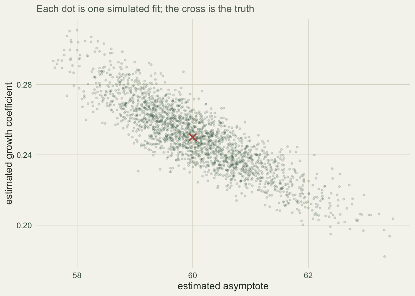
That trade-off is harmless when the oldest animals have levelled off, because the plateau pins \(L_\infty\) down. It becomes serious when they have not.
Refitting to fish aged six and under, which are still on the steep part of the curve, gives an asymptote of 53.4, and its standard error jumps from 0.9 on the full data to 2.8.
se_Ly  <- summary(fity)$coefficients["Linf", "Std. Error"]
wald_Ly <- coef(fity)["Linf"] + c(-1, 1) * 1.96 * se_Ly
prof_Ly <- suppressMessages(confint(fity, "Linf"))
The naive symmetric interval from that standard error runs 48.1 to 58.8, against a true asymptote of 60. The profile interval, 49.2 to 60.9, is the one to report, because the likelihood for an asymptote is skewed when the data stop short of it. Either way the message is the same: you cannot estimate a maximum size from animals that have not approached it, and nls will return a confident-looking number that is really an extrapolation. Report the asymptote with its profile interval, check whether your oldest ages have levelled off, and treat a maximum size projected from young individuals as a guess about a shape you have not observed. The next post is about exactly this: getting starting values and telling when a parameter is well determined.
References
- von Bertalanffy 1938 Human Biology 10(2):181-213 (pre-DOI; JSTOR 41447359)
- Walford 1946 Biological Bulletin 90(2):141-147 (10.2307/1538217)
- Ricker 1975, Computation and Interpretation of Biological Statistics of Fish Populations, Bulletin of the Fisheries Research Board of Canada 191
- Katsanevakis 2006 Fisheries Research 81(2-3):229-235 (10.1016/j.fishres.2006.07.002)
- Gallucci and Quinn 1979 Transactions of the American Fisheries Society 108(1):14-25 (10.1577/1548-8659(1979)108<14:RFATAS>2.0.CO;2)
- Ogle 2016, Introductory Fisheries Analyses with R, CRC Press (ISBN 978-1-4822-3520-3)
- Bates and Watts 1988, Nonlinear Regression Analysis and Its Applications, Wiley (ISBN 978-0-471-81643-0)