library(ggplot2)
library(patchwork)
te_paper  <- "#f5f4ee"
te_ink    <- "#16241d"
te_body   <- "#2c3a31"
te_forest <- "#275139"
te_rust   <- "#b5534e"
te_gold   <- "#c9b458"
te_line   <- "#dad9ca"
theme_datasheet <- function() {
  theme_minimal(base_size = 12) +
    theme(plot.background  = element_rect(fill = te_paper, colour = NA),
          panel.background = element_rect(fill = te_paper, colour = NA),
          panel.grid.major = element_line(colour = te_line, linewidth = 0.3),
          panel.grid.minor = element_blank(),
          text             = element_text(colour = te_body),
          plot.title       = element_text(colour = te_ink, face = "bold"),
          plot.subtitle    = element_text(colour = te_body),
          axis.text        = element_text(colour = te_body))
}Resource competition and the R-star rule
R
competition
coexistence
theoretical ecology
ecology tutorial
Tilman resource competition in R: a hand written RK4 chemostat shows why the lowest equilibrium resource level wins, and when two resources allow coexistence.
Two diatoms are grown together in one continuous culture. A single nutrient is scarce, everything else is supplied in excess, fresh medium flows in and culture flows out at a fixed rate, and cells are counted day after day. One of the two divides faster in fresh medium, and it dominates the opening weeks of the mixed culture by a wide margin. Then it stops increasing, turns over, and disappears. The slower species ends up owning the vessel. Tilman 1977 ran that contest with two freshwater diatoms competing for silicate and phosphate, and the winner was the one that held the limiting nutrient at the lower concentration.
The quantity that decides the contest is not the maximum growth rate and not the starting density. It is the concentration at which a species can just replace its losses, the level it drags the nutrient down to when it is alone and at equilibrium. Tilman 1982 called it R-star, and the criterion is that on one limiting resource the species with the lowest R-star excludes every other species, whatever their maximum rates, because the maximum rate enters only through the R-star it produces. That criterion is the head term of this post. Everything below is built to measure it, to find the point where it changes hands, and to see what survives when a second resource is added.
Bistability turns up in the second half, and here it is a consequence rather than a subject. The site already has a post on it: priority effects and alternative stable states shows that mutually strong competition produces two attractors and lets the arrival order pick between them. What is added below is where that strong mutual competition comes from. It is not assumed; it is produced by choosing which resource each consumer draws down hardest.
The two coexistence posts on the site sit on the other side of the same question. Fitting annual plant competition models estimates Beverton-Holt competition coefficients from a response surface, and those coefficients are phenomenological: fitted descriptions of how a plant’s fecundity falls when a neighbour is added, silent about what the neighbour took. Niche and fitness differences then computes a niche difference and a fitness difference from those fitted numbers. Here the mechanism is specified first and the competition coefficient comes out of the resource dynamics rather than out of a fit, and one section below shows what that derivation says about the niche difference when there is only one resource to divide. The tools are small on purpose: base R, stats and ggplot2, with a fixed step fourth order Runge-Kutta scheme written out in the post, and no differential equation package.
A consumer draws its resource to one level and holds it there
The chemostat is the cleanest setting for this because the losses are known exactly. Medium enters at dilution rate \(D\) carrying resource at supply concentration \(S\), culture leaves at the same rate, so every consumer loses a fraction \(D\) of itself per unit time whatever else happens. With the saturating uptake function Monod 1949 measured in bacterial cultures, the system for two consumers on one resource is
\[\frac{dR}{dt} = D(S - R) - \sum_i q_i \mu_i(R) N_i, \qquad \frac{dN_i}{dt} = N_i \left( \mu_i(R) - D \right), \qquad \mu_i(R) = \frac{r_i R}{K_i + R}\]
with \(r_i\) the maximum growth rate, \(K_i\) the half saturation constant and \(q_i\) the resource drawn per unit of consumer produced. Setting the second equation to zero gives the equilibrium resource level of species \(i\) on its own,
\[R^*_i = \frac{K_i D}{r_i - D}\]
which exists only when \(r_i > D\). Both the maximum rate and the half saturation constant enter it, so a species can reach a low \(R^*\) either by growing fast or by being efficient when the resource is scarce. Hsu, Hubbell and Waltman 1977 proved that in this system the species with the smallest \(R^*\) takes over from any positive starting densities, so what follows is a measurement of a result that is already known exactly, which is the right way to test an integrator.
rk4_run <- function(f, x0, h, nstep, keep) {
  x <- x0; out <- matrix(0, floor(nstep / keep) + 1, length(x0))
  tvec <- numeric(nrow(out)); out[1, ] <- x; j <- 1
  for (i in seq_len(nstep)) {
    k1 <- f(x); k2 <- f(x + (h / 2) * k1); k3 <- f(x + (h / 2) * k2); k4 <- f(x + h * k3)
    x <- x + (h / 6) * (k1 + 2 * k2 + 2 * k3 + k4)
    if (i %% keep == 0) { j <- j + 1; out[j, ] <- x; tvec[j] <- i * h }
  }
  list(tvec = tvec[seq_len(j)], x = out[seq_len(j), , drop = FALSE])
}
monod <- function(res, rmax, halfk) rmax * res / (halfk + res)
rstar_of <- function(rmax, halfk, loss) halfk * loss / (rmax - loss)
dil <- 0.25; sup_one <- 50; n_start <- 0.05  # dilution, supply, inoculum
h_fine <- 0.01; h_sweep <- 0.02; h_bi <- 0.05; h_two <- 0.1  # production steps
rmax_s <- 0.55; half_s <- 3                  # slow species: rate, half saturation
rmax_f <- 1.10; half_f <- 30                 # fast species: rate, half saturation
use_s <- 1; use_f <- 1                       # resource drawn per unit of consumer
rs_slow <- rstar_of(rmax_s, half_s, dil)
rs_fast <- rstar_of(rmax_f, half_f, dil); rate_ratio <- rmax_f / rmax_s
r_cross <- (rmax_s * half_f - rmax_f * half_s) / (rmax_f - rmax_s)
mu_at_supply <- c(monod(sup_one, rmax_s, half_s), monod(sup_one, rmax_f, half_f))
one_deriv <- function(rm_fast) function(x) {
  res <- x[1]; n_s <- x[2]; n_f <- x[3]
  g_s <- monod(res, rmax_s, half_s); g_f <- monod(res, rm_fast, half_f)
  c(dil * (sup_one - res) - use_s * g_s * n_s - use_f * g_f * n_f,
    n_s * (g_s - dil), n_f * (g_f - dil))
}
The fast species has 2.0 times the maximum growth rate of the slow one, and at the supply concentration it grows at 0.688 per day against 0.519 per day, so it really is the faster of the two where the experiment starts. Its half saturation constant is the price: the two growth curves cross at a resource concentration of 24.0, and below that the slow species grows faster. The closed form equilibrium levels are 2.500 for the slow species and 8.824 for the fast one. A hand written solver is a hypothesis until it is tested, so it is checked twice before anything rests on it: against a quantity with a closed form, and against itself at a finer step.
alone_s <- rk4_run(one_deriv(rmax_f), c(sup_one, n_start, 0), h_fine, 60000, 1000)
alone_f <- rk4_run(one_deriv(rmax_f), c(sup_one, 0, n_start), h_fine, 60000, 1000)
eq_err_s <- abs(alone_s$x[nrow(alone_s$x), 1] - rs_slow)
eq_err_f <- abs(alone_f$x[nrow(alone_f$x), 1] - rs_fast)
h_conv <- c(4, 2, 1) * h_fine
conv <- lapply(h_conv, function(h)
  rk4_run(one_deriv(rmax_f), c(sup_one, n_start, n_start), h, 200 / h, 1 / h))
gap_1 <- max(abs(conv[[1]]$x[, 2] - conv[[2]]$x[, 2]))
gap_2 <- max(abs(conv[[2]]$x[, 2] - conv[[3]]$x[, 2]))
gap_ratio <- gap_1 / gap_2; order_expected <- 2^4
Each species grown alone settles on the resource level its formula predicts, to within 1.217e-13 for the slow species and 3.268e-13 for the fast one. Halving the step twice shrinks the discrepancy between successive solutions from 7.592e-09 to 4.793e-10, a factor of 15.8 against the 16 that fourth order convergence predicts. That test covers the one resource runs, which use steps of 0.01 and 0.02 day, both inside the range it spans. The two resource work later is coarser, 0.05 day for the trajectories and 0.10 day for the outcome labelling, and it runs on a vector field with a kink in it where the limiting resource changes, so each half of it is checked against a finer step of its own in the section that uses it.
The faster species loses
Both species are inoculated at the same density into a vessel full of fresh medium, and the culture is followed until one of them is gone.
traj_one <- rk4_run(one_deriv(rmax_f), c(sup_one, n_start, n_start), h_fine, 40000, 25)
one_dat <- data.frame(day = traj_one$tvec, res = traj_one$x[, 1],
                      slow = traj_one$x[, 2], fast = traj_one$x[, 3])
end_row <- one_dat[nrow(one_dat), ]; peak_i <- which.max(one_dat$fast)
peak_fast <- one_dat$fast[peak_i]; peak_day <- one_dat$day[peak_i]
lead_at_peak <- one_dat$fast[peak_i] / one_dat$slow[peak_i]
ext_frac <- 0.01; ext_level <- n_start * ext_frac
ext_day <- one_dat$day[which(one_dat$fast < ext_level & one_dat$day > peak_day)[1]]
sim_rstar <- end_row$res; eq_dens <- (sup_one - rs_slow) / use_s
decline_rate <- dil - monod(rs_slow, rmax_f, half_f)
The fast species does win the early part of the experiment, and by a clear margin. It peaks on day 19.2 at 34.9 units of biomass, 5.6 times the density of the slow species at that moment. By then the resource has been pulled below the crossover concentration of 24.0, and from that point the ranking of the two growth rates is reversed for good. The fast species falls below 1 per cent of its inoculum on day 97 and keeps falling at 0.165 per day in log density, which is the dilution rate minus its Monod growth rate at the resource level the winner holds.
dens_long <- data.frame(day = rep(one_dat$day, 2), dens = c(one_dat$slow, one_dat$fast),
  species = rep(c("slow, low R-star", "fast, high R-star"), each = nrow(one_dat)))
p_dens <- ggplot(dens_long, aes(day, dens, colour = species)) + geom_line(linewidth = 0.9) +
  geom_hline(yintercept = ext_level, linetype = "dashed", colour = te_body, linewidth = 0.4) +
  scale_colour_manual(values = c(te_rust, te_forest), name = NULL) +
  scale_y_log10() + coord_cartesian(xlim = c(0, 220), ylim = c(1e-5, 200)) +
  labs(x = "day", y = "density (log scale)", title = "Densities",
       subtitle = "dashed: one per cent of the inoculum") +
  theme_datasheet() + theme(legend.position = "bottom")
p_res <- ggplot(one_dat, aes(day, res)) + geom_line(linewidth = 0.9, colour = te_ink) +
  geom_hline(yintercept = r_cross, linetype = "dotted", colour = te_gold, linewidth = 0.7) +
  geom_hline(yintercept = rs_fast, linetype = "dashed", colour = te_rust, linewidth = 0.6) +
  geom_hline(yintercept = rs_slow, colour = te_forest, linewidth = 0.6) +
  coord_cartesian(xlim = c(0, 220)) +
  labs(x = "day", y = "resource concentration", title = "Resource",
       subtitle = "dotted: the growth curves cross") + theme_datasheet()
p_dens + p_res + plot_annotation(theme = theme_datasheet())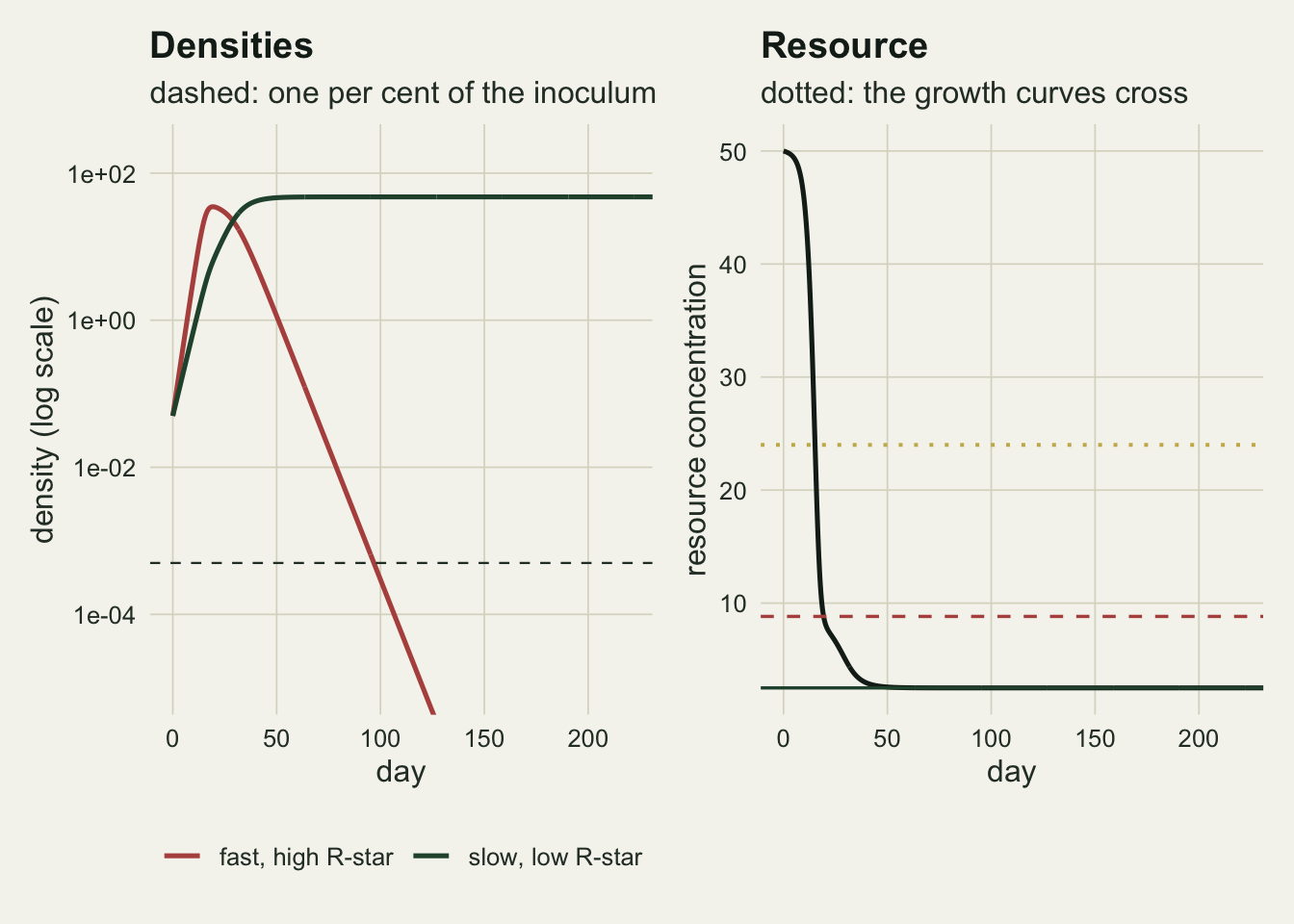
The culture settles at a resource concentration of 2.5000 against the closed form 2.5000 for the winner, and the winner’s density settles at 47.50 against the 47.50 that the resource budget forces. That agreement is the calibration: the simulation and the algebra are describing the same equilibrium.
Raising the loser’s maximum rate changes nothing until it changes R-star
The obvious objection is that the fast species was not fast enough. The formula answers it. Raising \(r_i\) does lower \(R^*_i\), but only through the difference \(r_i - D\) in the denominator. Setting the two equilibrium levels equal and solving for the maximum rate gives the point where the ranking changes hands, and that point can also be located from the simulations alone, by tracking the rate at which the loser’s share of the culture declines.
rmax_flip <- dil + half_f * dil / rs_slow
flip_ratio <- rmax_flip / rmax_s; sweep_tmax <- 600
sweep_rates <- seq(rmax_s * 1.2, rmax_s * 7, length.out = 11)
run_pair <- function(rm_fast, tmax = sweep_tmax, h = h_sweep)
  rk4_run(one_deriv(rm_fast), c(sup_one, n_start, n_start), h,
          round(tmax / h), round(1 / h))
share_slope <- function(z, lo = 400, hi = 600) {   # late trend in log(fast/slow)
  w <- which(z$tvec >= lo & z$tvec <= hi)
  as.numeric(coef(lm(log(z$x[w, 3]) - log(z$x[w, 2]) ~ z$tvec[w]))[2])
}
sweep_tab <- do.call(rbind, lapply(sweep_rates, function(rm_fast) {
  z <- run_pair(rm_fast); fin <- z$x[nrow(z$x), ]
  data.frame(rmax_fast = rm_fast, rstar_fast = rstar_of(rm_fast, half_f, dil),
             end_res = fin[1], end_slow = fin[2], end_fast = fin[3], slope = share_slope(z))
}))
sweep_tab$winner <- ifelse(sweep_tab$end_slow > sweep_tab$end_fast,
                           "slow species", "fast species")
sweep_tab$res_gap <- abs(sweep_tab$end_res - pmin(sweep_tab$rstar_fast, rs_slow))
rmax_flip_sim <- uniroot(function(rm_fast) share_slope(run_pair(rm_fast)),
                         c(rmax_s * 4, rmax_s * 8), tol = 1e-5)$root
flip_gap <- abs(rmax_flip_sim - rmax_flip) / rmax_flip
quad_row <- sweep_tab[which.min(abs(sweep_tab$rmax_fast - 4 * rmax_s)), ]
quad_vs_fast <- quad_row$rmax_fast / rmax_f; quad_vs_slow <- quad_row$rmax_fast / rmax_s
flip_vs_fast <- rmax_flip / rmax_f
worst_i <- which.max(sweep_tab$res_gap); res_worst <- sweep_tab$res_gap[worst_i]
res_rest <- max(sweep_tab$res_gap[-worst_i])
slow_slope <- abs(sweep_tab$slope[worst_i]); worst_holder <- sweep_tab$winner[worst_i]
worst_dir <- ifelse(sweep_tab$slope[worst_i] < 0, "falling", "rising")
Raising the fast species maximum growth rate to 2.26 per day, 2.05 times the rate it already had and 4.1 times the slow species rate, leaves the outcome untouched: the slow species still ends with 47.5 units against 8.55e-16, and the culture still settles at a resource concentration of 2.500. The exchange happens at a maximum rate of 3.250000 per day from the formula and 3.250002 per day from the simulations, a relative gap of 6.10e-07. That crossing rate is 5.91 times the slow species maximum rate and 2.95 times the rate the fast species already has, so the loser has to reach nearly six times the slow species maximum rate before the sign of its long run advantage changes, and what changes at that point is not its speed but its \(R^*\).
line_dat <- data.frame(rmax_fast = seq(min(sweep_rates), max(sweep_rates), length.out = 300))
line_dat$rstar_fast <- rstar_of(line_dat$rmax_fast, half_f, dil)
ggplot(line_dat, aes(rmax_fast, rstar_fast)) +
  geom_line(colour = te_rust, linewidth = 0.9) +
  geom_hline(yintercept = rs_slow, colour = te_forest, linewidth = 0.8) +
  geom_vline(xintercept = rmax_flip, linetype = "dotted",
             colour = te_body, linewidth = 0.6) +
  geom_point(data = sweep_tab, aes(rmax_fast, end_res, colour = winner), size = 2.6) +
  scale_colour_manual(values = c(te_rust, te_forest), name = "survivor") +
  coord_cartesian(ylim = c(0, 9)) +
  labs(x = "maximum growth rate of the fast species (per day)",
       y = "resource concentration", title = "R-star, not speed, decides the contest",
       subtitle = "red curve: the fast species R-star; green line: the slow species R-star") +
  theme_datasheet() + theme(legend.position = "bottom")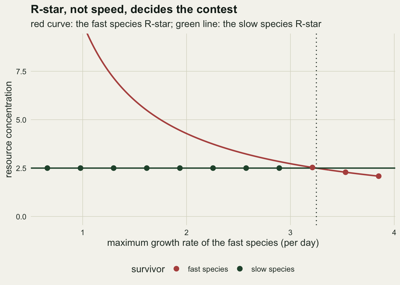
The points are the resource concentrations the simulated mixed cultures actually settle at, and they sit on the lower of the two curves everywhere except at the run closest to the crossing, where the gap reaches 0.032. At that maximum rate the two equilibrium levels differ by so little that the loser is being displaced at 0.0017 per day in log density, and the 600 day horizon is not long enough to finish the job. The survivor colour at that one point is an artefact of that horizon: it reads fast species because that species still holds the higher density on the last day, while the log ratio of fast to slow there is already falling. Every other run sits on the lower curve to within 2.452e-04.
One resource leaves no room for a niche difference
The competition coefficients that the annual plant post fits can be derived here instead. If the resource equilibrates quickly relative to the consumers, then \(R\) is a function of the two densities, and the per capita growth rate of each species inherits a dependence on both. Differentiating the resource balance implicitly and dividing the interspecific sensitivity by the intraspecific one gives
\[\alpha_{ij} = \frac{q_j \mu_j(R)}{q_i \mu_i(R)}\]
rspan <- seq(rs_slow, sup_one, length.out = 400)
alpha_sf <- (use_f * monod(rspan, rmax_f, half_f)) / (use_s * monod(rspan, rmax_s, half_s))
alpha_fs <- 1 / alpha_sf
prod_dev  <- max(abs(alpha_sf * alpha_fs - 1))
niche_dev <- max(abs(1 - sqrt(alpha_sf * alpha_fs)))
alpha_at_win <- alpha_sf[1]
The product \(\alpha_{ij}\alpha_{ji}\) is one at every resource concentration in the run, with a largest deviation of 1.110e-16, which is floating point noise. In the notation of the niche and fitness post the niche difference is one minus the square root of that product, so it is 1.110e-16: zero by construction, everywhere. The two species overlap completely, because there is only one thing to overlap on. The individual coefficients are neither one nor equal: at the resource level the winner holds, the fast species presses on the slow one with 0.338 of the strength the slow species presses on itself, which reads as stabilising until the reciprocal coefficient is read beside it. With no niche difference the outcome is entirely a fitness difference, and on one resource the fitness difference is the R-star ranking. Coexistence needs a second resource, and it needs more than merely having one.
Two resources coexist only where the consumption vectors match
Give the two consumers two essential resources, so that growth follows the minimum of the two Monod terms rather than their product, and let each species be the better competitor for one of them. That trade-off puts a corner on each zero net growth isocline, the two isoclines cross at one point, and the supply then decides the rest. The geometry is the one Tilman 1980 set out.
rmx <- 1.0
half_sp1 <- c(3, 12)     # species 1: good on resource 1, poor on resource 2
half_sp2 <- c(12, 3)     # species 2: the mirror image
cons_sp1 <- c(0.3, 0.7)  # species 1 takes mostly resource 2
cons_sp2 <- c(0.7, 0.3)  # species 2 takes mostly resource 1
rst_sp1 <- half_sp1 * dil / (rmx - dil)   # zero net growth corner, species 1
rst_sp2 <- half_sp2 * dil / (rmx - dil)   # and species 2
res_int <- c(rst_sp2[1], rst_sp1[2])      # where the two isoclines cross
grow_two <- function(rr, halfk)
  rmx * min(rr[1] / (halfk[1] + rr[1]), rr[2] / (halfk[2] + rr[2]))
two_deriv <- function(c1, c2, spl) function(x) {
  rr <- pmax(x[1:2], 0); n1 <- x[3]; n2 <- x[4]
  g1 <- grow_two(rr, half_sp1); g2 <- grow_two(rr, half_sp2)
  c(dil * (spl[1] - rr[1]) - c1[1] * g1 * n1 - c2[1] * g2 * n2,
    dil * (spl[2] - rr[2]) - c1[2] * g1 * n1 - c2[2] * g2 * n2,
    n1 * (g1 - dil), n2 * (g2 - dil))
}
mono_eq <- function(rst, cvec, spl) {
  n_a <- (spl[1] - rst[1]) / cvec[1]; n_b <- (spl[2] - rst[2]) / cvec[2]
  if (n_a > 0 && spl[2] - cvec[2] * n_a >= rst[2])
    return(c(rst[1], spl[2] - cvec[2] * n_a, n_a))
  if (n_b > 0 && spl[1] - cvec[1] * n_b >= rst[1])
    return(c(spl[1] - cvec[1] * n_b, rst[2], n_b))
  c(spl[1], spl[2], 0)
}
label_cell <- function(c1, c2, spl) {
  e1 <- mono_eq(rst_sp1, c1, spl); e2 <- mono_eq(rst_sp2, c2, spl)
  ok1 <- e1[3] > 0; ok2 <- e2[3] > 0
  if (!ok1 || !ok2) return(if (ok1) "species 1 wins" else
                           if (ok2) "species 2 wins" else "neither persists")
  inv1 <- grow_two(e2[1:2], half_sp1) - dil   # invasion of a species 2 stand
  inv2 <- grow_two(e1[1:2], half_sp2) - dil   # invasion of a species 1 stand
  if (inv1 > 0 && inv2 > 0) return("coexistence")
  if (inv1 < 0 && inv2 < 0) return("bistable")
  if (inv1 > 0) "species 1 wins" else "species 2 wins"
}
sup_seq <- seq(3.3, 31.3, length.out = 15)
cell_tab <- expand.grid(s1 = sup_seq, s2 = sup_seq); n_cell <- nrow(cell_tab)
spl_i <- function(i) c(cell_tab$s1[i], cell_tab$s2[i])   # the supply pair of one cell
lab_col <- function(c1, c2)
  vapply(seq_len(n_cell), function(i) label_cell(c1, c2, spl_i(i)), "")
cell_tab$matched <- lab_col(cons_sp1, cons_sp2)
cell_tab$swapped <- lab_col(cons_sp2, cons_sp1)
sup_lo <- min(sup_seq); sup_hi <- max(sup_seq)
n_coex <- sum(cell_tab$matched == "coexistence")
n_bist <- sum(cell_tab$swapped == "bistable")
pct_coex <- 100 * n_coex / n_cell; pct_bist <- 100 * n_bist / n_cell
same_set <- identical(which(cell_tab$matched == "coexistence"),
                      which(cell_tab$swapped == "bistable"))
The isoclines cross at a resource pair of 4.0 and 4.0. There species 1 is limited by resource 2 and species 2 by resource 1, each by the resource it is worse at, and the consumption vectors are set so that each consumer takes more of the resource that limits it. On a 15 by 15 grid of supply points running from 3.3 to 31.3 in each resource, 114 of the 225 cells give coexistence, which is 50.7 per cent of the grid. Those labels come from the mutual invasion criterion evaluated at monoculture equilibria in closed form, so they deserve a second and independent determination. The check integrates the full four dimensional system from two starting points, one at each monoculture equilibrium with the other species introduced at a trace density, and reads the label off the state the trajectory reaches.
persist_at <- 1e-3
sim_label <- function(c1, c2, spl, h = h_two, tmax = 600, trace_d = 1e-4) {
  e1 <- mono_eq(rst_sp1, c1, spl); e2 <- mono_eq(rst_sp2, c2, spl)
  f <- two_deriv(c1, c2, spl)
  x1 <- if (e1[3] > 0) c(e1[1:2], e1[3], trace_d) else c(spl, trace_d, trace_d)
  x2 <- if (e2[3] > 0) c(e2[1:2], trace_d, e2[3]) else c(spl, trace_d, trace_d)
  z1 <- rk4_run(f, x1, h, tmax / h, tmax / h)$x[2, ]
  z2 <- rk4_run(f, x2, h, tmax / h, tmax / h)$x[2, ]
  code_of <- function(e) paste0(as.integer(e[3] > persist_at), as.integer(e[4] > persist_at))
  if (code_of(z1) != code_of(z2)) return("bistable")
  switch(code_of(z1), "11" = "coexistence", "10" = "species 1 wins",
         "01" = "species 2 wins", "00" = "neither persists")
}
set.seed(41)
n_per_class <- 6
check_i <- unlist(lapply(split(seq_len(n_cell), cell_tab$matched),
  function(v) v[sample(length(v), min(n_per_class, length(v)))]))
h_two_fine <- h_two / 4
check_m <- vapply(check_i, function(i) sim_label(cons_sp1, cons_sp2, spl_i(i)), "")
check_s <- vapply(check_i, function(i) sim_label(cons_sp2, cons_sp1, spl_i(i)), "")
long_m <- vapply(check_i, function(i)
  sim_label(cons_sp1, cons_sp2, spl_i(i), tmax = 1200), "")
fine_m <- vapply(check_i, function(i)
  sim_label(cons_sp1, cons_sp2, spl_i(i), h = h_two_fine), "")
n_check <- length(check_i); moved_long <- sum(long_m != check_m)
moved_fine <- sum(fine_m != check_m)
agree_m <- sum(check_m == cell_tab$matched[check_i])
agree_s <- sum(check_s == cell_tab$swapped[check_i])
Of the 19 sampled cells, six from each outcome class that had six to give, the simulation reproduces the closed form label in 19 cells under matched consumption and 19 under swapped consumption. Doubling the integration horizon on the matched runs moves 0 labels, and cutting their step to 0.025 day, a quarter of the production step, moves 0. So those trajectories are being read at their attractors rather than in transit, and the coarse step is not what decides the labels on a vector field that has a kink in it.
zngi_arm <- function(rst, tagname, hi)
  data.frame(x = c(rst[1], rst[1], hi), y = c(hi, rst[2], rst[2]), who = tagname)
hi_lim <- max(sup_seq) + 2
zngi_all <- rbind(zngi_arm(rst_sp1, "species 1", hi_lim),
                  zngi_arm(rst_sp2, "species 2", hi_lim))
arrow_of <- function(ca, cb) data.frame(
  x = res_int[1], y = res_int[2], who = c("species 1", "species 2"),
  xend = res_int[1] + 9 * c(ca[1], cb[1]), yend = res_int[2] + 9 * c(ca[2], cb[2]))
out_cols <- c("coexistence" = te_gold, "bistable" = te_gold, "neither persists" = te_ink,
              "species 1 wins" = te_forest, "species 2 wins" = te_rust)
map_plot <- function(col_name, arrows, ttl) {
  ggplot(cell_tab, aes(s1, s2)) +
    geom_point(aes(colour = .data[[col_name]]), size = 2.2) +
    geom_path(data = zngi_all, aes(x, y, group = who, linetype = who),
              colour = te_body, linewidth = 0.7) +
    geom_segment(data = arrows, aes(x = x, y = y, xend = xend, yend = yend,
                 linetype = who), colour = te_ink, linewidth = 0.6,
                 arrow = arrow(length = unit(0.16, "cm"), type = "closed")) +
    scale_colour_manual(values = out_cols, name = NULL) +
    scale_linetype_manual(values = c("solid", "dashed"), guide = "none") +
    guides(colour = guide_legend(nrow = 2)) +
    labs(x = "supply of resource 1", y = "supply of resource 2", title = ttl) +
    theme_datasheet() + theme(legend.position = "bottom",
      legend.box = "vertical", legend.key.size = unit(0.3, "cm"),
      legend.text = element_text(size = 7.5), legend.margin = margin(1, 1, 1, 1))
}
map_plot("matched", arrow_of(cons_sp1, cons_sp2), "Matched consumption vectors") +
  labs(subtitle = "arrows: each species consumption vector at the crossing point")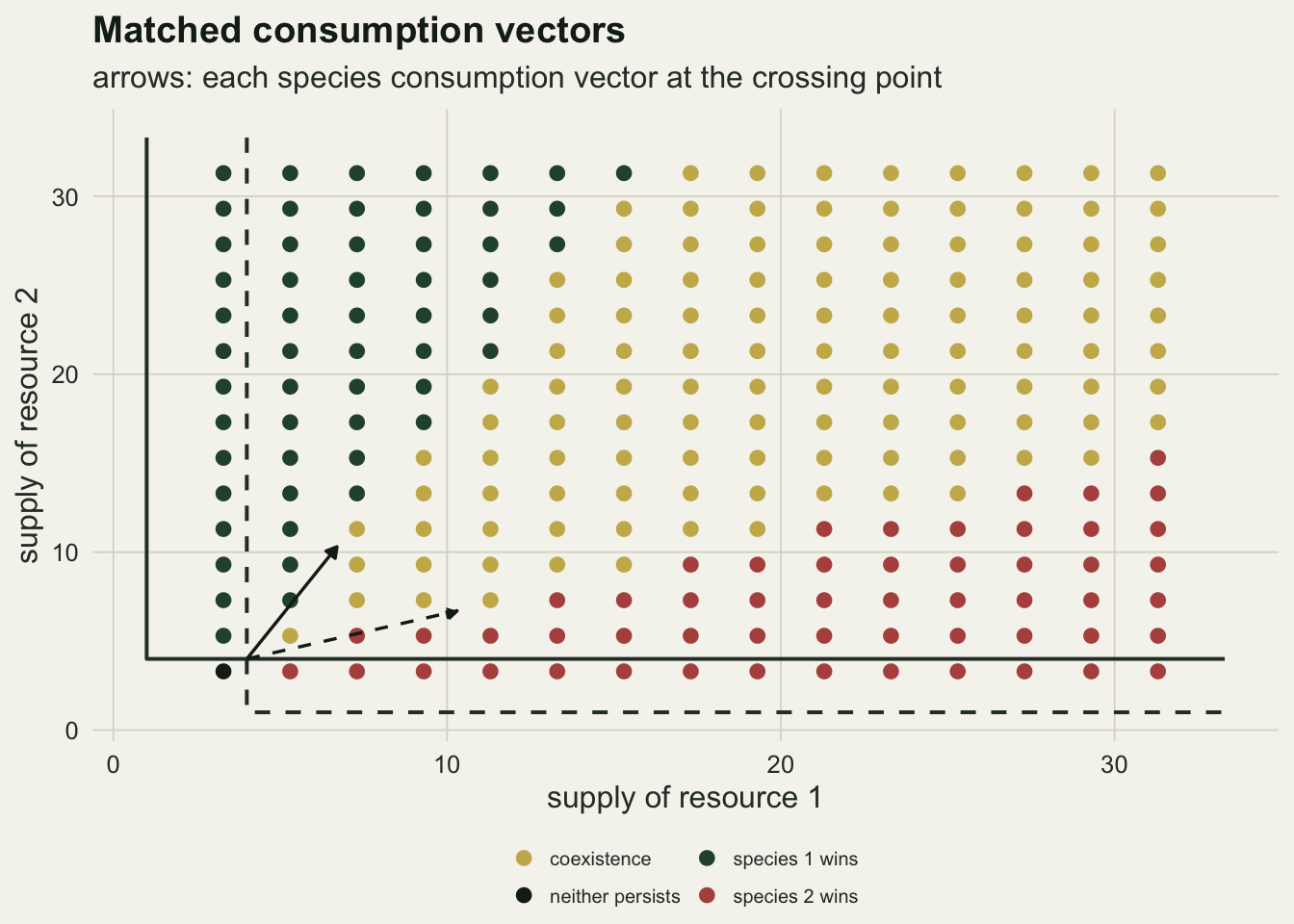
The gold wedge is the set of supply points that can be written as the crossing point plus a positive combination of the two consumption vectors, and that is the entire content of the coexistence condition. Outside it the supply is too lopsided for one of the species to hold a positive density, and the winner is whichever the supply favours.
The same wedge turns bistable when the vectors are swapped
Now change one thing. Leave the isoclines, the half saturation constants, the maximum rates and the dilution rate exactly as they are, and swap the consumption vectors, so that each species takes more of the resource that limits its competitor rather than the one that limits itself. The interior equilibrium does not move: the isoclines are unchanged, so the crossing point is where it was. What can change is its stability, and the linearisation says so before any trajectory is drawn.
sup_bi <- c(15.3, 19.3)
dens_m <- solve(cbind(cons_sp1, cons_sp2), sup_bi - res_int)
dens_int <- solve(cbind(cons_sp2, cons_sp1), sup_bi - res_int)
jac_num <- function(f, x, eps = 1e-6) vapply(seq_along(x), function(j) {
  bump <- numeric(length(x)); bump[j] <- eps
  (f(x + bump) - f(x - bump)) / (2 * eps)
}, numeric(length(x)))
lead_of <- function(c1, c2, nn)
  max(Re(eigen(jac_num(two_deriv(c1, c2, sup_bi), c(res_int, nn)))$values))
lead_m <- lead_of(cons_sp1, cons_sp2, dens_m); lead_s <- lead_of(cons_sp2, cons_sp1, dens_int)
head_hi <- 0.50; head_lo <- 0.05
bi_run <- function(n1, n2) rk4_run(two_deriv(cons_sp2, cons_sp1, sup_bi),
                                   c(sup_bi, n1, n2), h_bi, 12000, 100)
bi_one <- bi_run(head_hi, head_lo); bi_two <- bi_run(head_lo, head_hi)
end_1 <- bi_one$x[nrow(bi_one$x), ]; end_2 <- bi_two$x[nrow(bi_two$x), ]
head_start <- head_hi / head_lo
bi_half <- rk4_run(two_deriv(cons_sp2, cons_sp1, sup_bi), c(sup_bi, head_hi, head_lo),
                   h_bi / 2, 24000, 200)
bi_dev <- abs(bi_half$x[nrow(bi_half$x), 3] / end_1[3] - 1)
Take a supply of 15.3 in resource 1 and 19.3 in resource 2, which is one of the grid cells inside the wedge. The interior equilibrium there holds the resources at the crossing point under either set of consumption vectors, with the two consumers at 8.30 and 18.30 units under the swapped ones. The leading eigenvalue of the numerically differentiated Jacobian at that equilibrium is -0.1978 per day with matched vectors and 0.2234 per day with swapped vectors, so the same interior point is an attractor in one case and a saddle in the other.
traj_of <- function(z, tag) rbind(
  data.frame(day = z$tvec, dens = z$x[, 3], species = "species 1", start = tag),
  data.frame(day = z$tvec, dens = z$x[, 4], species = "species 2", start = tag))
traj_bi <- rbind(traj_of(bi_one, "species 1 first"), traj_of(bi_two, "species 2 first"))
p_traj <- ggplot(traj_bi, aes(day, dens, colour = species, linetype = start)) +
  geom_line(linewidth = 0.8) +
  scale_colour_manual(values = c(te_forest, te_rust), name = NULL) +
  scale_linetype_manual(values = c("solid", "dashed"), name = NULL) +
  scale_y_log10() + coord_cartesian(ylim = c(1e-6, 100)) +
  labs(x = "day", y = "density (log scale)", title = "Same supply, two outcomes") +
  theme_datasheet() + theme(legend.position = "bottom",
    legend.box = "vertical", legend.key.width = unit(0.9, "cm"),
    legend.text = element_text(size = 7.5), legend.margin = margin(1, 1, 1, 1))
map_plot("swapped", arrow_of(cons_sp2, cons_sp1), "Swapped vectors") + p_traj +
  plot_annotation(theme = theme_datasheet())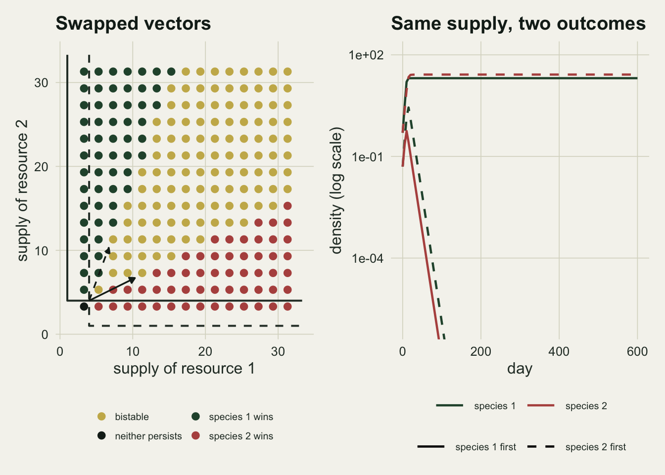
Two runs at that supply point, identical except for which species starts with a 10 fold density advantage, end in different places. Starting species 1 ahead leaves it at 20.43 units with species 2 at 2.83e-45; starting species 2 ahead leaves species 2 at 26.14 with species 1 at 3.31e-44. The survivors hold the resources at different levels too, 1.00 and 13.17 in the first case against 7.46 and 1.00 in the second. Halving the step of these two runs to 0.025 day moves the surviving density at the end of the first by a relative 7.33e-15.
Across the whole grid 114 cells are bistable under swapped consumption, 50.7 per cent of it, and they are the identical set of supply points that gave coexistence with matched vectors. Nothing about the species pair changed except which resource each draws down hardest, and the same region of supply space went from holding both species to holding whichever one arrived first. That is the mechanistic version of the founder control the priority effects post reaches through assumed Lotka-Volterra competition coefficients.
What to report
Report the equilibrium resource level each species holds on its own, together with the parameters it was computed from. An \(R^*\) without its loss rate is not a number anyone can reuse, because it is a property of the species and the loss rate together, and a species that wins at one dilution rate can lose at another. Report the maximum growth rates as well, and say plainly whether they decided anything. The most useful single sentence in a resource competition result is the one naming the species with the higher maximum rate and the species that won, when those differ. If they are the same species the experiment has not separated the two explanations, and it should be presented that way. With two or more resources, report the consumption vectors and not only the isoclines. The isoclines fix where coexistence is possible; the consumption vectors fix whether the interior equilibrium is stable, and the same isoclines support coexistence or founder control depending only on them. Half saturation constants with no consumption stoichiometry are half a model. Report the supply point too, and where it sits relative to the coexistence region: two experiments that disagree about whether a pair coexists may simply have used different medium.
Honest limits
The chemostat is the reason the argument is this clean. Every consumer loses individuals at exactly the dilution rate, so the loss term is known rather than estimated and \(R^*\) has a closed form. In a lake or a soil the loss rate mixes grazing, sinking and mortality, it differs between species and it varies through the season, and the equivalent of \(R^*\) then depends on a quantity that is itself hard to measure. Miller and colleagues 2005 went through the papers citing the resource ratio theory and found only a few dozen well designed tests of its predictions, most of them in laboratory microcosms with freshwater algae rather than in the field. Growth is also treated as a function of the current external concentration, which is the Monod form. Many algae and plants store nutrients internally and grow on the internal quota instead, which decouples uptake from growth and can carry a species through a spell when the external level sits below the \(R^*\) computed from a steady state experiment. Droop’s quota model is the standard repair, and Grover 1997 works through what quota dynamics do to the competition criterion.
The two resource section uses essential resources with a strict minimum, the sharpest version of the geometry. Substitutable resources give straight isoclines, and perfectly substitutable ones remove the corner and with it most of the room for coexistence. The corner is doing real work here, and it is a modelling assumption rather than an observation. Everything else is deterministic, continuous and homogeneous. There is no demographic stochasticity, so the loser declines forever without reaching zero, and the extinction time above is the time to cross a threshold that was chosen rather than measured. A finite population would have gone extinct earlier and by a different mechanism.
The grid percentages depend on the grid. A coexistence share of 50.7 per cent describes the particular square of supply space sampled here, from 3.3 to 31.3 in each resource, and it would change if that square were moved or stretched. What does not depend on the grid is the shape of the region: a wedge with its apex at the isocline crossing and its edges along the two consumption vectors. The grid was also offset so that no supply point falls exactly on an edge of that wedge, where the outcome is a knife edge and either label is defensible.
References
Monod J 1949 Annual Review of Microbiology 3:371-394 (10.1146/annurev.mi.03.100149.002103)
Tilman D 1977 Ecology 58(2):338-348 (10.2307/1935608)
Tilman D 1980 The American Naturalist 116(3):362-393 (10.1086/283633)
Tilman D 1982 Resource Competition and Community Structure (ISBN 978-0-691-08302-5)
Hsu SB, Hubbell SP, Waltman P 1977 SIAM Journal on Applied Mathematics 32(2):366-383 (10.1137/0132030)
Grover JP 1997 Resource Competition (ISBN 978-0-412-74930-8)
Miller TE, Burns JH, Munguia P, Walters EL, Kneitel JM, Richards PM, Mouquet N, Buckley HL 2005 The American Naturalist 165(4):439-448 (10.1086/428681)