library(ggplot2)
library(patchwork)

te_paper  <- "#f5f4ee"
te_ink    <- "#16241d"
te_body   <- "#2c3a31"
te_forest <- "#275139"
te_rust   <- "#b5534e"
te_gold   <- "#c9b458"
te_line   <- "#dad9ca"

theme_datasheet <- function() {
  theme_minimal(base_size = 12) +
    theme(plot.background  = element_rect(fill = te_paper, colour = NA),
          panel.background = element_rect(fill = te_paper, colour = NA),
          panel.grid.major = element_line(colour = te_line, linewidth = 0.3),
          panel.grid.minor = element_blank(),
          text             = element_text(colour = te_body),
          plot.title       = element_text(colour = te_ink, face = "bold"),
          plot.subtitle    = element_text(colour = te_body),
          axis.text        = element_text(colour = te_body))
}The paradox of enrichment in R
R
theoretical ecology
population dynamics
predation
ecology tutorial
Enrichment in R: a Rosenzweig-MacArthur model integrated by hand, the Hopf point located twice, and a limit cycle trough far below one surviving animal.
A fenced reserve of four hundred hectares carries a herbivore at about one animal per hectare, a few hundred head in total, and a predator that lives on it. The reserve is then enriched: fertiliser runoff from the neighbouring farm, a wetter decade, or a manager who stops mowing, and the forage that sets the herbivore’s carrying capacity quadruples. The obvious expectation is more herbivores. What the standard predator and prey model predicts is that the herbivore’s average density rises roughly in step with the forage, the predator does well, and the trough of the resulting cycle drops to a density at which the whole reserve holds less than a ten thousandth of one animal.
That last clause is what this post measures. The functional responses post ends by asserting that a type II response is destabilising and can drive prey to local extinction, but it stops there: that post fits the disc equation to feeding trial counts and never runs the dynamics the shape implies. Here the dynamics are run, the destabilisation is located as a number, and the depth of the trough is converted into animals.
The tools are already in use on this site. A fixed step fourth order Runge-Kutta scheme written out by hand appears in the SEIR model and latency, and linearising about an equilibrium and reading the leading eigenvalue appears in seasonality and recurrent epidemics. Neither is the lesson here. What is new is the kind of boundary. The site’s existing tipping point material is about a fold, where two equilibria collide and annihilate and the state jumps to a distant branch, and the seasonality post crosses a forced period doubling, where an annual cycle becomes biennial. A Hopf bifurcation is neither of those. Nothing collides and nothing doubles: a single equilibrium stays exactly where it is and merely stops attracting, while a cycle of growing amplitude appears around it.
A predator that saturates, integrated in logarithms
The model is Rosenzweig and MacArthur’s. Prey grow logistically towards a carrying capacity, and the predator eats them through a Holling type II functional response, so its intake saturates at one over the handling time however many prey are on offer.
\[\frac{dN}{dt} = r N \left(1 - \frac{N}{K}\right) - \frac{a N P}{1 + a h N}, \qquad \frac{dP}{dt} = \frac{e a N P}{1 + a h N} - m P\]
The integration is done on the logarithms of the two densities rather than on the densities themselves. That is not cosmetic. The whole point of this post is a trough many orders of magnitude below the mean, and a scheme stepping a linear state variable will eventually take a density negative down there, after which the run is fiction. In logarithms the state cannot cross zero, and the relative accuracy at the trough is the same as the relative accuracy at the peak.
rk4_log <- function(deriv, x0, dt_h, nstep, keep) {
  y <- log(x0)
  out <- matrix(0, floor(nstep / keep) + 1, length(x0))
  tt <- numeric(nrow(out)); out[1, ] <- x0; j <- 1
  for (i in seq_len(nstep)) {
    k1 <- deriv(exp(y)); k2 <- deriv(exp(y + (dt_h / 2) * k1))
    k3 <- deriv(exp(y + (dt_h / 2) * k2)); k4 <- deriv(exp(y + dt_h * k3))
    y <- y + (dt_h / 6) * (k1 + 2 * k2 + 2 * k3 + k4)
    if (i %% keep == 0) { j <- j + 1; out[j, ] <- exp(y); tt[j] <- i * dt_h }
  }
  list(t = tt[seq_len(j)], x = out[seq_len(j), , drop = FALSE])
}

r_prey <- 0.5; att <- 1.0; handle <- 0.45; conv <- 0.3; mort <- 0.2
dt_h <- 0.05; burn_t <- 6000; meas_t <- 4000; intake_cap <- 1 / handle

n_star <- mort / (att * (conv - mort * handle))
p_star_of <- function(kk) (r_prey / att) * (1 - n_star / kk) * (1 + att * handle * n_star)

rm_log <- function(kk) function(z) {
  n <- z[1]; p <- z[2]
  c(r_prey * (1 - n / kk) - att * p / (1 + att * handle * n),
    conv * att * n / (1 + att * handle * n) - mort)
}

run_k <- function(kk, x0 = NULL, burn = burn_t, meas = meas_t, hh = dt_h, out_dt = 0.5) {
  if (is.null(x0)) x0 <- c(n_star * 1.05, p_star_of(kk))
  z <- rk4_log(rm_log(kk), x0, hh, round((burn + meas) / hh), round(out_dt / hh))
  sel <- z$t > burn; nn <- z$x[sel, 1]
  list(nmin = min(nn), navg = mean(nn), npeak = max(nn), amp = (max(nn) - min(nn)) / 2,
       endstate = z$x[nrow(z$x), ], tt = z$t[sel], nn = nn, pp = z$x[sel, 2])
}

print(round(c(prey_r = r_prey, attack = att, handling = handle, conversion = conv,
              death = mort, ceiling = intake_cap, step = dt_h, window = meas_t), 4))
prey_r attack handling conversion death ceiling step
0.5000 1.0000 0.4500 0.3000 0.2000 2.2222 0.0500
window
4000.0000 Every run below uses those settings. Prey increase at 0.50 per unit time, the attack rate is 1.0, the handling time is 0.45 so the predator cannot eat more than 2.22 prey per unit time however many are available, 0.30 of a prey becomes predator, and predators die at 0.20 per unit time. The step is 0.05, the default burn-in is 6000 time units and the measurement window that follows it is 4000.
Nothing in this post is stochastic, so there is no seed and no replication: one run per parameter value, reproducible to the last digit. The burn-in was not chosen by eye either. Close to the boundary located below, the transient decays at a rate that approaches zero, so the amplitude runs near it are given a burn-in scaled to their own decay rate from the linearisation rather than the default, which is generous everywhere else and would be far too short there.
The integrator is a hypothesis until it is checked
Three checks, none of which the scheme can pass by accident. The first uses a case with a known conserved quantity: strip the carrying capacity and the handling time and the model collapses to Lotka and Volterra’s, whose orbits lie on the level sets of a function mixing both densities. The integrator knows nothing about that function, so any drift in it is pure truncation error. The second halves the step on the cycle that matters and watches the trough. The third varies the interval at which output is stored, because a minimum is only ever read off the points that were kept.
lv_log <- function(z) c(r_prey - att * z[2], conv * att * z[1] - mort)
lv_inv <- function(n, p) conv * att * n - mort * log(n) + att * p - r_prey * log(p)

lv_steps <- c(0.2, 0.1, 0.05)
lv_drift <- vapply(lv_steps, function(hh) {
  z <- rk4_log(lv_log, c(0.5, 0.4), hh, round(2000 / hh), round(1 / hh))
  v <- lv_inv(z$x[, 1], z$x[, 2])
  max(abs(v - v[1])) / abs(v[1])
}, 0)
lv_ratio <- lv_drift[-length(lv_drift)] / lv_drift[-1]

k_show    <- 16
halve_min <- vapply(c(0.2, 0.1, 0.05, 0.025), function(hh) run_k(k_show, hh = hh)$nmin, 0)
halve_rel <- abs(diff(halve_min)) / halve_min[-1]
res_rel   <- abs(run_k(k_show, out_dt = dt_h)$nmin - halve_min[3]) / halve_min[3]
sig_keep  <- floor(-log10(max(halve_rel[2], halve_rel[3], res_rel)))

print(signif(lv_drift, 4)); print(round(lv_ratio, 2)); print(signif(halve_rel, 3))
[1] 1.827e-07 5.649e-09 1.727e-10[1] 32.34 32.72[1] 5.71e-05 3.06e-06 1.93e-07The Lotka-Volterra invariant drifts by 1.73e-10 of itself over two thousand time units at the production step, and each halving of the step cuts that drift by a factor of 32.3 and then 32.7. Those factors are larger than the sixteen that a fourth order global error would give, which is what a closed orbit should do: the error committed per step is of order the fifth power of the step, and around a loop it does not accumulate secularly, so the drift over a fixed horizon falls faster than the global error bound. On the cycle itself the trough moves by 3.06e-06 of itself when the step is halved to the production value, and by 1.93e-07 on the next halving, and storing the state ten times more often moves it by 7.62e-07, so the minimum reported below is a property of the trajectory and not of the output grid. Those two checks pin the trough to 5 significant figures, and nothing below is quoted beyond that.
Enrichment leaves the prey equilibrium exactly where it was
Setting the predator equation to zero gives the interior equilibrium prey density directly: intake must exactly pay the predator’s death rate, which fixes the prey density at the death rate divided by the attack rate times the difference between conversion efficiency and the product of death rate and handling time. The carrying capacity does not appear anywhere in it. Whatever the forage does, the prey density at which a predator population breaks even is a property of the predator.
k_stable  <- c(1.5, 2, 2.5, 3, 3.5, 4)
stable_nb <- vapply(k_stable, function(kk) run_k(kk)$navg, 0)
stable_pb <- vapply(k_stable, function(kk) mean(run_k(kk)$pp), 0)
n_spread  <- max(stable_nb) - min(stable_nb)
p_gain    <- stable_pb[length(stable_pb)] / stable_pb[1]
k_gain    <- k_stable[length(k_stable)] / k_stable[1]

print(data.frame(K = k_stable, prey = signif(stable_nb, 9), predator = signif(stable_pb, 6)))
K prey predator
1 1.5 0.952381 0.260771
2 2.0 0.952381 0.374150
3 2.5 0.952381 0.442177
4 3.0 0.952381 0.487528
5 3.5 0.952381 0.519922
6 4.0 0.952381 0.544218Raising the carrying capacity by a factor of 2.67 moves the settled prey density across those six runs by 5.83e-12, which is the integrator’s arithmetic and not a response. Over the same range the predator equilibrium rises by a factor of 2.09, from 0.261 to 0.544. Every unit of extra production goes to the predator. That is Rosenzweig and MacArthur’s graphical result, and it is already odd enough before anything becomes unstable: fertilise the field and the herbivore gains nothing at all.
The Hopf point, located twice
The next claim needs a number rather than a glance at a time series, so the boundary is located twice. The first route is the linearisation. Build the two by two Jacobian at the interior equilibrium and track the largest real part of its eigenvalues as the carrying capacity moves. Where that real part changes sign, the equilibrium stops attracting, and a bracketed root find returns the crossing to whatever precision the eigenvalue solver supports.
The second is the simulation. Above a supercritical Hopf point the amplitude of the emerging cycle grows like the square root of the distance from the boundary, so the squared amplitude is locally linear in the carrying capacity and extrapolates to zero at it. Measure the squared amplitude at five capacities above the boundary, fit a straight line, and read off its root. Each run after the first starts from the final state of the run before it, so settling onto each cycle is a short correction rather than slow growth away from the equilibrium.
jac_at <- function(kk) {
  fprime <- att / (1 + att * handle * n_star)^2
  fofn   <- att * n_star / (1 + att * handle * n_star)
  pp     <- p_star_of(kk)
  matrix(c(r_prey - 2 * r_prey * n_star / kk - pp * fprime, conv * pp * fprime,
           -fofn, conv * fofn - mort), 2, 2)
}
jac_re <- function(kk) max(Re(eigen(jac_at(kk))$values))

k_lin      <- uniroot(jac_re, c(2, 10), tol = 1e-10)$root
k_analytic <- 2 * n_star + 1 / (att * handle)
k_gap_form <- abs(k_lin - k_analytic)
eig_crit   <- eigen(jac_at(k_lin))$values
cyc_period <- 2 * pi / abs(Im(eig_crit)[1])

print(signif(c(k_linearisation = k_lin, k_closed_form = k_analytic), 10))
k_linearisation k_closed_form
4.126984 4.126984 print(signif(eig_crit, 6))[1] 0+0.232048i 0-0.232048ik_amp <- c(4.2, 4.3, 4.4, 4.5, 4.6)
amp_obs <- numeric(length(k_amp)); warm <- NULL
for (i in seq_along(k_amp)) {
s <- run_k(k_amp[i], x0 = warm, burn = 25 / jac_re(k_amp[i]), meas = 3000)
amp_obs[i] <- s$amp; warm <- s$endstate
}
fit_amp <- lm(amp_obs^2 ~ k_amp)
k_sim <- unname(-coef(fit_amp)[1] / coef(fit_amp)[2])
amp_r2 <- summary(fit_amp)$r.squared
k_hopf_gap <- k_sim - k_lin; k_hopf_pct <- 100 * k_hopf_gap / k_lin
win_lo <- min(k_amp) - k_lin; win_hi <- max(k_amp) - k_lin
print(data.frame(K = k_amp, amplitude = signif(amp_obs, 6), squared = signif(amp_obs^2, 6))) K amplitude squared
1 4.2 0.374679 0.140384
2 4.3 0.580435 0.336905
3 4.4 0.733741 0.538376
4 4.5 0.863040 0.744839
5 4.6 0.977926 0.956340print(signif(c(k_simulation = k_sim, k_linearisation = k_lin), 8)) k_simulation k_linearisation
4.133622 4.126984 The linearisation puts the boundary at 4.126984. This model happens to admit a closed form as well, because the equilibrium loses stability exactly when it falls to the left of the hump in the prey nullcline, which happens at twice the equilibrium prey density plus one over the product of attack rate and handling time. That expression evaluates to 4.126984 and differs from the root find by 2.38e-11, so the eigenvalue route is doing its arithmetic correctly.
At the crossing the leading pair is 0.232048 times the imaginary unit and its conjugate, with a real part at the root finder’s tolerance. A complex pair crossing the imaginary axis is the signature of a Hopf bifurcation, and it is what separates this boundary from the fold in the tipping points post, where a single real eigenvalue passes through zero and no oscillation is implied. The imaginary part sets the period of the cycle that is born, 27.08 time units. May’s paper on limit cycles in predator and prey communities is the reason to expect a bounded cycle here rather than a spiral running away to the axes, and the amplitudes measured next are what a bounded cycle looks like.
The amplitude route puts the boundary at 4.133622. The straight line through the five squared amplitudes has an R squared of 0.99979, which is the square root law behaving as advertised. The two estimates differ by 0.006638, or 0.16 per cent of the boundary value, and the sign of the difference is the expected one: the fitted window sits between 0.07 and 0.47 above the boundary, where the square root law is only asymptotic, so the extrapolation lands slightly high. Agreement to within a fifth of one per cent from two routes that share the equations and the starting point but nothing in the estimate itself is the reason the numbers below can be quoted at all.
k_fine <- seq(2, 8, length.out = 250)
lin_df <- data.frame(K = k_fine, re = vapply(k_fine, jac_re, 0))
p_lin <- ggplot(lin_df, aes(K, re)) +
  geom_hline(yintercept = 0, colour = te_rust, linewidth = 0.5) +
  geom_vline(xintercept = k_lin, colour = te_gold, linetype = "dashed", linewidth = 0.7) +
  geom_line(colour = te_forest, linewidth = 0.9) +
  labs(x = "carrying capacity K", y = "leading real part", title = "Linearisation",
       subtitle = "gold: eigenvalue sign change") +
  theme_datasheet()

amp_df  <- data.frame(K = k_amp, sq = amp_obs^2)
pred_df <- data.frame(K = seq(k_sim, max(k_amp), length.out = 100))
pred_df$sq <- predict(fit_amp, newdata = data.frame(k_amp = pred_df$K))
p_amp <- ggplot(amp_df, aes(K, sq)) +
  geom_hline(yintercept = 0, colour = te_rust, linewidth = 0.5) +
  geom_line(data = pred_df, aes(K, sq), colour = te_forest, linewidth = 0.8) +
  geom_point(size = 2.8, colour = te_ink) +
  geom_vline(xintercept = k_sim, colour = te_gold, linetype = "dashed", linewidth = 0.7) +
  scale_x_continuous(limits = c(k_sim - 0.03, max(k_amp) + 0.05)) +
  labs(x = "carrying capacity K", y = "squared cycle amplitude", title = "Simulation",
       subtitle = "gold: root of the fitted line") +
  theme_datasheet()

p_lin + p_amp + plot_annotation(theme = theme_datasheet())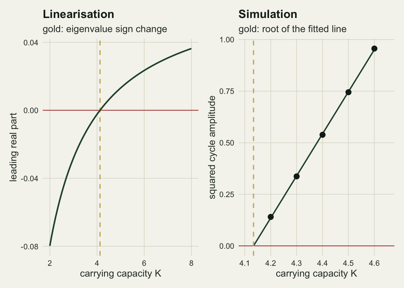
The average rises and the trough falls off a cliff
With a boundary in hand, sweep the carrying capacity across it and record three summaries of the prey series after the burn-in: its time average, its peak and its minimum.
k_grid <- c(seq(1.5, 4, by = 0.5), 4.2, 4.5, 5, 6, 7, 8, 10, 12, 14, 16, 18, 20)
sweep_raw <- vapply(k_grid, function(kk) {
  s <- run_k(kk); c(s$nmin, s$navg, s$npeak)
}, numeric(3))
sweep_df <- setNames(data.frame(k_grid, t(sweep_raw)), c("K", "nmin", "navg", "npeak"))

above    <- sweep_df$K > k_lin
avg_expo <- unname(coef(lm(log(navg) ~ log(K), data = sweep_df[above, ]))[2])
min_dec  <- unname(coef(lm(log10(nmin) ~ K, data = sweep_df[above, ]))[2])
quad_fac <- 4^avg_expo

k_low <- 3; k_high <- 16; low_run <- run_k(k_low); high_run <- run_k(k_high)
avg_ratio <- high_run$navg / low_run$navg
min_ratio <- low_run$nmin / high_run$nmin
gap_ratio <- high_run$navg / high_run$nmin

print(signif(as.matrix(sweep_df[sweep_df$K %in% c(3, 4, 4.5, 6, 8, 12, 16, 20), ]), 6))
K nmin navg npeak
4 3.0 9.52381e-01 0.952381 0.952381
6 4.0 9.52381e-01 0.952381 0.952381
8 4.5 3.36421e-01 1.062700 2.062500
10 6.0 4.86335e-02 1.489940 4.279900
12 8.0 4.68519e-03 2.025030 6.781690
14 12.0 3.42900e-05 3.047430 11.406700
16 16.0 1.84729e-07 4.114160 15.739800
18 20.0 8.11469e-10 5.296910 19.895500print(round(c(mean_exponent = avg_expo, log10_min_per_K = min_dec), 4)) mean_exponent log10_min_per_K
1.0665 -0.5519 Below the boundary the three summaries coincide, because the trajectory has settled on the equilibrium and a constant has no peak and no trough. Above it they separate, and they separate at completely different rates. The time average grows as the carrying capacity raised to the power 1.07, so above the boundary multiplying the forage by four multiplies the average number of prey alive by 4.39. The minimum falls by 0.55 orders of magnitude for every unit added to the carrying capacity, with no sign of levelling off at the top of the sweep.
In terms of the two example capacities, going from 3 to 16 multiplies the prey time average by 4.32 and divides the cycle minimum by 5.16e+06. The average is a fair description of a settled population and a misleading one here: the series it summarises spends part of every cycle at a density 2.23e+07 times below it. This is the part of the paradox that survives measurement. The often repeated version, that enrichment leaves mean prey density unchanged, is exactly true only below the boundary, where the equilibrium does not move at all; above it the mean does rise, and what collapses is the minimum.
patch_area <- 400; floor_dens <- 1 / patch_area; win_t <- 300
cyc_lab <- c(sprintf("K = %g (below the boundary)", k_low),
             sprintf("K = %g (above the boundary)", k_high))
cyc_df <- rbind(
  data.frame(t = low_run$tt - burn_t, n = low_run$nn, run = cyc_lab[1]),
  data.frame(t = high_run$tt - burn_t, n = high_run$nn, run = cyc_lab[2]))
cyc_df <- cyc_df[cyc_df$t <= win_t, ]
cyc_df$run <- factor(cyc_df$run, levels = cyc_lab)

ggplot(cyc_df, aes(t, n, colour = run)) +
  geom_hline(yintercept = floor_dens, colour = te_body, linetype = "dashed", linewidth = 0.5) +
  geom_line(linewidth = 0.8) +
  scale_colour_manual(values = c(te_forest, te_rust), name = NULL) +
  scale_y_log10(breaks = 10^seq(-8, 2, by = 2),
                labels = c("1e-08", "1e-06", "1e-04", "0.01", "1", "100")) +
  labs(x = "time", y = "prey density (per hectare)",
       title = "Only one of these is a population",
       subtitle = "dashed: the density at which 400 hectares hold a single animal") +
  theme_datasheet() +
  theme(legend.position = "bottom")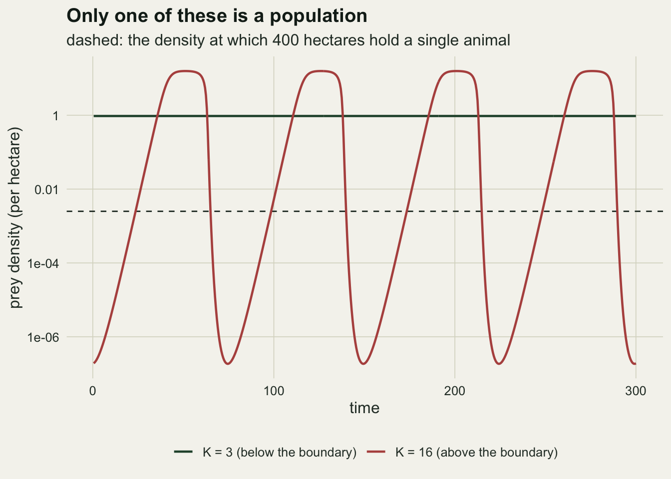
What the trough is worth in animals
A density is not an outcome. Attach the model to the reserve from the opening: four hundred hectares, prey densities read as animals per hectare. There is then a density below which the reserve holds less than one animal, namely one over its area, and the question is where the cycle minimum sits relative to it.
ind_low_min  <- low_run$nmin * patch_area
ind_high_avg <- high_run$navg * patch_area
ind_high_min <- high_run$nmin * patch_area
ind_high_pk  <- high_run$npeak * patch_area
ind_capacity <- k_high * patch_area
floor_factor <- floor_dens / high_run$nmin

k_ext <- uniroot(function(kk) log(run_k(kk)$nmin) - log(floor_dens), c(6, 11), tol = 1e-3)$root
k_ext_mult <- k_ext / k_lin

print(round(c(capacity = ind_capacity, low_trough = ind_low_min,
              high_average = ind_high_avg, high_peak = ind_high_pk), 1))
capacity low_trough high_average high_peak
6400.0 381.0 1645.7 6295.9 print(signif(c(individuals_high_trough = ind_high_min, K_at_one_individual = k_ext), 6))individuals_high_trough K_at_one_individual
7.38918e-05 8.52813e+00 At the low carrying capacity the reserve holds 381 prey and holds them steadily. At the high one the forage would support 6400, the herd averages 1646 and peaks at 6296, which is what an enrichment programme would be judged on, and once per cycle it passes through a trough of 7.39e-05 animals. The trough density is 13533 times below the density at which the reserve contains one individual. The equations do not notice, because a differential equation is content to carry a ten thousandth of an animal through the winter and rebuild a herd from it. A reserve is not.
That gives a second threshold, and a more useful one than the Hopf point. Solving for the carrying capacity at which the cycle minimum first falls below one animal in the reserve gives 8.53, which is 2.07 times the Hopf value. Between those two numbers the model oscillates and the oscillation is survivable. Past 8.53 the deterministic attractor is a cycle whose low point is extinction, and calling that attractor stable is a statement about the equations rather than about the herbivore. Mollison made the same objection in an epidemic setting when he named the atto-fox: a compartmental model has no smallest unit, so it recovers happily from a population that cannot exist. Gilpin’s reply to Rosenzweig raised it for enrichment specifically, within a year of the paper that named the paradox.
long_df <- rbind(
  data.frame(K = sweep_df$K, value = sweep_df$navg, what = "time average"),
  data.frame(K = sweep_df$K, value = sweep_df$nmin, what = "cycle minimum"))

ggplot(long_df, aes(K, value, colour = what)) +
  geom_hline(yintercept = floor_dens, colour = te_body, linetype = "dashed", linewidth = 0.5) +
  geom_vline(xintercept = k_lin, colour = te_gold, linetype = "dashed", linewidth = 0.7) +
  geom_line(linewidth = 0.9) +
  geom_point(size = 1.8) +
  scale_colour_manual(values = c(te_rust, te_forest), name = NULL) +
  scale_y_log10(breaks = 10^seq(-9, 1, by = 2),
                labels = c("1e-09", "1e-07", "1e-05", "0.001", "0.1", "10")) +
  labs(x = "carrying capacity K", y = "prey density (per hectare)",
       title = "Enrichment feeds the average and empties the trough",
       subtitle = "gold dashed: Hopf point; dark dashed: one animal in 400 hectares") +
  theme_datasheet() +
  theme(legend.position = "bottom")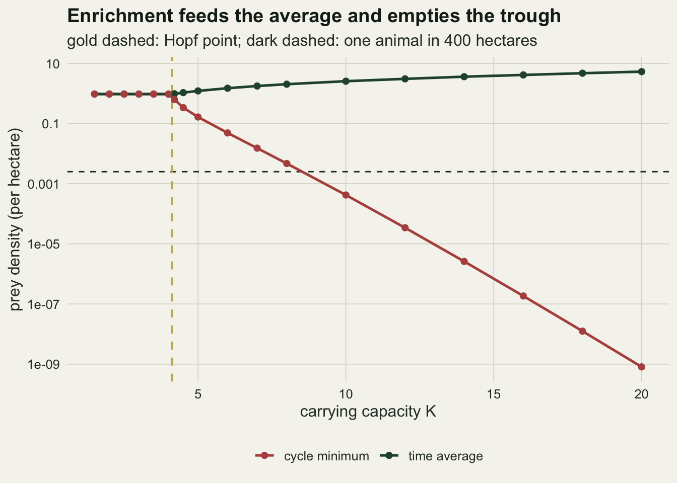
A type III response removes the boundary entirely
The destabilising ingredient is the shape of the functional response at low prey density. Under a type II response the per capita risk to a prey individual is highest when prey are rare, which is the mechanism the functional responses post described. A type III response reverses that: the predator is inefficient at low prey density, so rarity is a refuge. Keeping the attack rate, handling time, conversion and death rate identical and changing only the shape gives a nearly identical equilibrium prey density, which makes the comparison clean.
n3 <- sqrt(mort / (att * (conv - mort * handle)))

re_type3 <- function(kk) {
  fofn   <- att * n3^2 / (1 + att * handle * n3^2)
  fprime <- 2 * att * n3 / (1 + att * handle * n3^2)^2
  pp     <- r_prey * n3 * (1 - n3 / kk) / fofn
  max(Re(eigen(matrix(c(r_prey - 2 * r_prey * n3 / kk - pp * fprime, conv * pp * fprime,
                        -fofn, conv * fofn - mort), 2, 2))$values))
}

k_probe  <- c(seq(1.5, 30, by = 0.5), 60, 120, 240, 500, 1000); k_probe_lo <- min(k_probe)
re3_top  <- max(vapply(k_probe, re_type3, 0)); k_probe_top <- max(k_probe)

rm3_log <- function(kk) function(z) {
  n <- z[1]; p <- z[2]; fofn <- att * n^2 / (1 + att * handle * n^2)
  c(r_prey * (1 - n / kk) - fofn * p / n, conv * fofn - mort)
}
run3 <- function(kk) {
  fofn <- att * n3^2 / (1 + att * handle * n3^2)
  z <- rk4_log(rm3_log(kk), c(n3 * 1.05, r_prey * n3 * (1 - n3 / kk) / fofn),
               dt_h, round((burn_t + meas_t) / dt_h), round(0.5 / dt_h))
  nn <- z$x[z$t > burn_t, 1]
  c(nmin = min(nn), namp = (max(nn) - min(nn)) / 2)
}
t3_k    <- c(4, 16, 30)
t3_runs <- t(vapply(t3_k, run3, numeric(2)))
t3_amp  <- max(t3_runs[, "namp"]); t3_ind <- t3_runs[2, "nmin"] * patch_area
t3_amp_txt <- if (t3_amp == 0) "exactly zero" else formatC(t3_amp, format = "e", digits = 1)

print(signif(c(n_eq_type3 = n3, worst_real_part = re3_top, largest_K = k_probe_top), 6))
n_eq_type3 worst_real_part largest_K
0.975900 -0.100146 1000.000000 print(signif(t3_runs, 6)) nmin namp
[1,] 0.9759 0
[2,] 0.9759 0
[3,] 0.9759 0There is no boundary to find. Across every carrying capacity probed, from 1.5 up to 1000, the largest real part of the eigenvalue pair reaches -0.1001 at its worst, at the top of that range, and it approaches that ceiling from below instead of crossing zero. The simulations agree: at carrying capacities of 4, 16 and 30 the measured cycle amplitude is exactly zero to double precision, meaning the trajectory returns to the equilibrium and stays there, and the prey sit at 0.9759 per hectare, or 390 animals in the reserve, at every one of them.
The reason is in the nullclines. A type II prey nullcline is a hump, and enrichment pushes the hump to the right while the predator’s vertical nullcline stays put, so sooner or later the equilibrium ends up on the rising left arm where the feedback turns positive. A type III prey nullcline rises steeply as prey become rare, and with these parameters the equilibrium stays on a falling arm for any carrying capacity. Holling described both shapes in the paper that named them, and which one a particular predator shows at low prey density is the single most consequential feature in this model. It is also the hardest part of a functional response to estimate, for the reason that post gives: two curves that agree perfectly at the densities you sampled can imply opposite dynamics at the densities you did not.
k_cmp <- seq(1.6, 30, length.out = 300)
cmp_df <- rbind(
  data.frame(K = k_cmp, re = vapply(k_cmp, jac_re, 0), shape = "type II (saturating)"),
  data.frame(K = k_cmp, re = vapply(k_cmp, re_type3, 0), shape = "type III (sigmoid)"))

ggplot(cmp_df, aes(K, re, colour = shape)) +
  geom_hline(yintercept = 0, colour = te_body, linewidth = 0.5) +
  geom_line(linewidth = 0.9) +
  scale_colour_manual(values = c(te_forest, te_rust), name = NULL) +
  labs(x = "carrying capacity K", y = "leading real part",
       title = "Only one of these shapes has a Hopf point",
       subtitle = "identical attack rate, handling time, conversion and mortality") +
  theme_datasheet() +
  theme(legend.position = "bottom")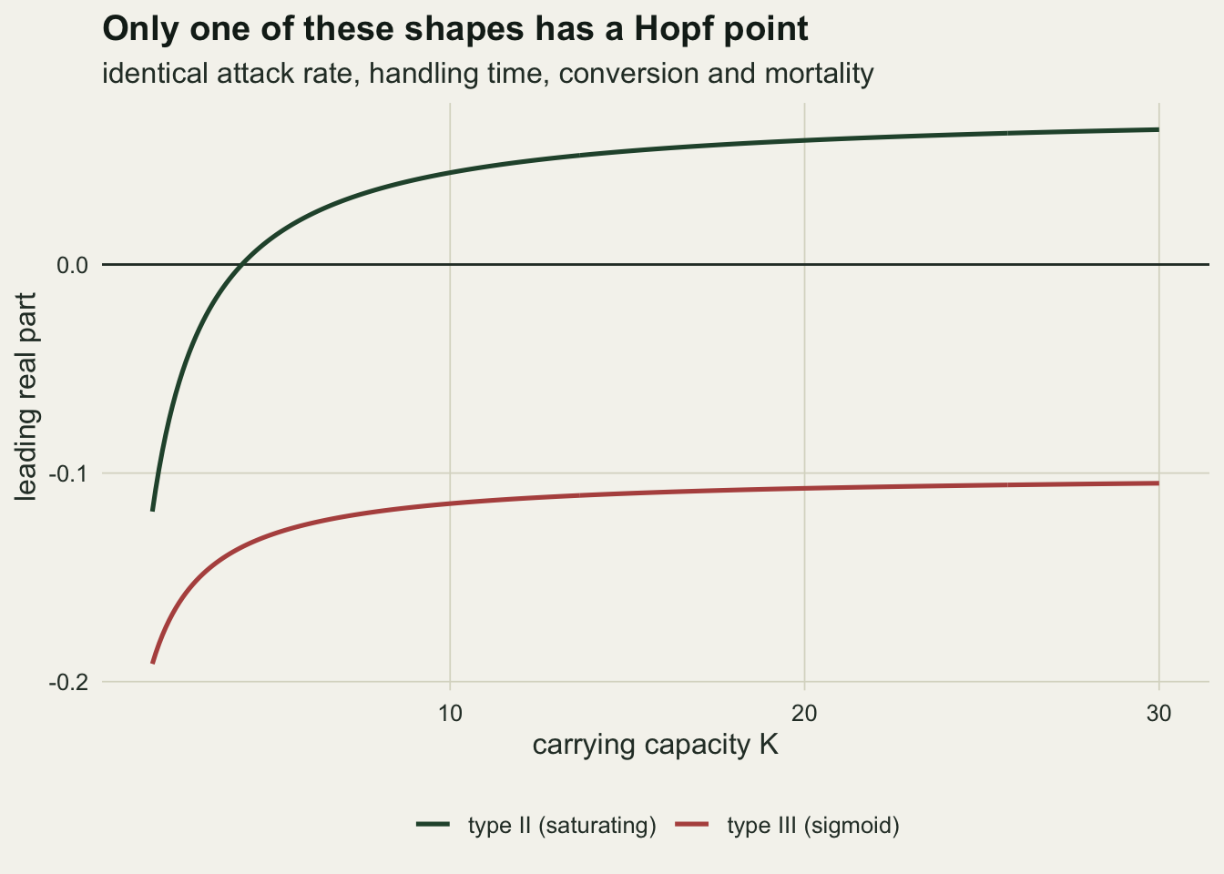
What to report
Give the boundary as a number and say how it was obtained. A statement that a model destabilises above some enrichment level is worth little without either an eigenvalue crossing or a fitted amplitude root behind it, and reporting both costs one extra function and catches the sign errors in a hand written Jacobian that a plotted time series will not.
Report the cycle minimum alongside the time average, always, and convert it into individuals using an explicit area or population size. A time average is the number a deterministic model makes look reasonable, and it is not the number that decides whether the population persists. If the minimum implies a fraction of an animal, say so plainly: the model has left the range in which its own units mean anything.
State the burn-in and how it was chosen, and state the step and the evidence that the answer does not depend on it. Near a Hopf point the transient decays at a rate that goes to zero, so a burn-in that was generous far from the boundary can be far too short close to it, and a cycle amplitude measured on an unconverged transient is an underestimate that happens to look smooth.
Say which functional response shape was assumed and what evidence supports it at low prey density. Everything measured above turns on that shape, and the difference between the two versions here is the difference between a population that oscillates into an impossible trough and one that does not oscillate at all.
Honest limits
The model has no stochasticity, no age structure, no space and no immigration. That is deliberate, because the argument is about what the deterministic skeleton predicts, but it means the extinction threshold computed here is a bound on the problem rather than an estimate of it. Demographic noise will finish a population long before the deterministic minimum reaches one individual, so the real threshold sits below the one measured above, not above it.
The translation into animals assumes the prey form one well mixed population across four hundred hectares. Space is the standard escape route from this paradox: Jansen showed that coupling patches by dispersal can keep an enriched predator and prey system persistent, because the patches drift out of phase and the metapopulation minimum is nowhere near the local one. None of that exists in a two variable model, and a reserve that is really a set of weakly connected patches will tolerate more enrichment than the number above suggests.
Prey growth is logistic and the carrying capacity is the only thing enrichment changes. Real enrichment usually changes the prey’s intrinsic rate of increase as well, changes which prey species dominates, and sometimes changes the predator’s handling time by changing prey quality. The closed form says which of those matter: the boundary is twice the equilibrium prey density plus one over the product of attack rate and handling time, so a shift in the foraging parameters moves it, while the prey growth rate does not enter it at all. A faster growing prey reaches the cycle sooner; it does not reach it at a different carrying capacity.
Early warning signals are a natural question here and this post does not answer it. The standard indicators are built for a real eigenvalue approaching zero, as at the fold in the tipping points post. At a Hopf the leading pair is complex, so the lag-1 autocorrelation of a sampled series depends on how the sampling interval compares with the period of the emerging oscillation, and an indicator can rise, fall or do neither depending on a choice made by the observer. Checking that properly needs a sweep over sampling intervals, which is a separate exercise and is not attempted above.
The depth of the trough is a real property of these equations, but its value is not a quantity anyone should transport. It depends on the parameters exponentially, as the sweep’s slope of 0.55 orders of magnitude per unit of carrying capacity shows, so a small change in the handling time or the predator’s death rate moves it by orders of magnitude. What transports is the shape of the result: an average that tracks enrichment, a minimum that does not, and a gap between them that widens without limit.
References
Rosenzweig ML 1971 Science 171(3969):385-387 (10.1126/science.171.3969.385)
Rosenzweig ML, MacArthur RH 1963 The American Naturalist 97(895):209-223 (10.1086/282272)
May RM 1972 Science 177(4052):900-902 (10.1126/science.177.4052.900)
Gilpin ME 1972 Science 177(4052):902-904 (10.1126/science.177.4052.902)
Holling CS 1959 The Canadian Entomologist 91(7):385-398 (10.4039/Ent91385-7)
Mollison D 1991 Mathematical Biosciences 107(2):255-287 (10.1016/0025-5564(91)90009-8)
Jansen VAA 1995 Oikos 74(3):384 (10.2307/3545983)