The SEIR model and the latent period

Add an exposed class to the SIR model in R, integrate it with a hand written RK4 solver, and measure how a latent period biases the reproduction number.

Almost no pathogen makes its host infectious the moment it arrives. Rabies takes weeks to reach the salivary glands, measles takes about a week and a half before the first cough, and even a fast respiratory virus in a wild bird colony needs a day or two of replication before the animal sheds anything. During that interval the host is infected, is not yet a source, and looks perfectly healthy to anyone counting sick animals. The SIR model has nowhere to put that host. It moves an individual from susceptible to infectious in the same instant.

The repair is one extra compartment. Call it E for exposed, meaning infected but not yet infectious, and let individuals leave it at rate sigma, so the average latent period is \(1/\sigma\). The model is then SEIR, and the question this post answers is what that extra box buys and what it costs. The answer is sharper than it first looks. The basic reproduction number does not move at all, and neither does the fraction of the population that is infected by the end. Every other quantity an epidemiologist actually measures in the field does move, and the worst consequence is quiet: a growth rate measured off a real outbreak and pushed through the SIR formula for \(R_0\) returns a number that is much too small, with no warning that anything is wrong.

This post assumes The SIR epidemic model, which sets up the compartments, the reproduction number and the final size relation. Here we integrate both models by hand with a fixed step fourth order Runge-Kutta scheme written out in the post, check the integrator before trusting it, and then measure the size of the inversion error for latent periods of two, five and ten days. The last two sections go after the assumption almost everyone makes without saying so, which is that the latent period is exponentially distributed, and then after the same assumption applied to the infectious period, where the error changes sign.

library(ggplot2)
library(grid)

te_pal <- list(forest = "#275139", green = "#2f8f63", sage = "#93a87f",
               clay = "#b5534e", gold = "#cda23f", line = "#dad9ca",
               ink = "#16241d", paper = "#f5f4ee")

theme_te <- function() {
  theme_minimal(base_size = 12) +
    theme(panel.grid.minor = element_blank(),
          panel.grid.major = element_line(colour = "#e7e6dc"),
          plot.background = element_rect(fill = "#f5f4ee", colour = NA),
          panel.background = element_rect(fill = "#f5f4ee", colour = NA),
          plot.title = element_text(face = "bold", colour = te_pal$ink),
          axis.title = element_text(colour = "#2c3a31"))
}

One set of equations for every model in the post

The SEIR system in fractions of the population is

\[\frac{dS}{dt} = -\beta S I, \quad \frac{dE}{dt} = \beta S I - \sigma E, \quad \frac{dI}{dt} = \sigma E - \gamma I, \quad \frac{dR}{dt} = \gamma I\]

with \(\beta\) the transmission rate, \(1/\sigma\) the mean latent period and \(1/\gamma\) the mean infectious period. Setting \(\sigma\) to infinity, which in practice means deleting the E box, recovers SIR.

Later we need two more variants: a latent period made of \(m\) sequential stages each with rate \(m\sigma\), and an infectious period made of \(n\) stages each with rate \(n\gamma\). Both keep the mean and shrink the variance. Rather than write four models, write one with the stage counts as arguments. The state vector is susceptibles, then the \(m\) latent stages, then the \(n\) infectious stages, then the removed class, and the derivative is assembled by shifting the outflow of each stage into the next.

stage_deriv <- function(beta, sigma, gamma, m, n) {
  function(x) {
    sus <- x[1]
    lat <- if (m > 0) x[1 + seq_len(m)] else numeric(0)
    inf <- x[1 + m + seq_len(n)]
    new <- beta * sus * sum(inf)
    if (m > 0) {
      out_e <- m * sigma * lat
      d_lat <- c(new, out_e[-m]) - out_e
      into_i <- out_e[m]
    } else {
      d_lat <- numeric(0)
      into_i <- new
    }
    out_i <- n * gamma * inf
    c(-new, d_lat, c(into_i, out_i[-n]) - out_i, out_i[n])
  }
}

rk4_run <- function(f, x0, h, nstep, keep) {
  x <- x0
  out <- matrix(0, floor(nstep / keep) + 1, length(x0))
  tt <- numeric(nrow(out))
  out[1, ] <- x
  j <- 1
  for (i in seq_len(nstep)) {
    k1 <- f(x)
    k2 <- f(x + (h / 2) * k1)
    k3 <- f(x + (h / 2) * k2)
    k4 <- f(x + h * k3)
    x <- x + (h / 6) * (k1 + 2 * k2 + 2 * k3 + k4)
    if (i %% keep == 0) {
      j <- j + 1
      out[j, ] <- x
      tt[j] <- i * h
    }
  }
  list(t = tt[seq_len(j)], x = out[seq_len(j), , drop = FALSE])
}

r0_true <- 2.5; inf_days <- 6; gam <- 1 / inf_days; bet <- r0_true * gam
seed <- 1e-6; step <- 0.01; horizon <- 500

epi <- function(lat_days, m = 1, n = 1, h = step, tmax = horizon, out_dt = 0.5) {
  if (lat_days == 0) m <- 0
  sig <- if (lat_days > 0) 1 / lat_days else 0
  x0 <- c(1 - seed, rep(0, m), seed, rep(0, n - 1), 0)
  z <- rk4_run(stage_deriv(bet, sig, gam, m, n), x0, h,
               round(tmax / h), round(out_dt / h))
  data.frame(t = z$t, S = z$x[, 1],
             prev = rowSums(z$x[, 1 + m + seq_len(n), drop = FALSE]),
             total = rowSums(z$x))
}

print(round(c(R0 = r0_true, infectious_period_days = inf_days, gamma = gam,
              beta = bet, seed_prevalence = seed, step_days = step,
              horizon_days = horizon), 6))

                    R0 infectious_period_days                  gamma 
              2.500000               6.000000               0.166667 
                  beta        seed_prevalence              step_days 
              0.416667               0.000001               0.010000 
          horizon_days 
            500.000000 

Every run in the post shares these settings. The reproduction number is 2.5, the mean infectious period is six days, so the recovery rate is 0.166667 per day and the transmission rate is 0.416667 per day. The epidemic is seeded with one infectious individual per million in an otherwise susceptible population, the step is 0.01 days and the horizon is 500 days, which is long enough for the slowest of these epidemics to finish.

Checking the integrator before believing anything it says

A hand written solver deserves two tests. The first is a conservation identity the scheme knows nothing about: the four compartments sum to one at every step, because every term in the derivative appears once positive and once negative. Runge-Kutta preserves that exactly in arithmetic, so any deviation is floating point error and nothing else. The second is convergence. A fourth order scheme has global error proportional to \(h^4\), so halving the step should shrink the difference between successive solutions by a factor of sixteen. Run the same epidemic three times at 0.05, 0.025 and 0.0125 days and compare the two gaps.

coarse <- epi(5, h = 0.05, tmax = 200)
mid <- epi(5, h = 0.025, tmax = 200)
fine <- epi(5, h = 0.0125, tmax = 200)
d1 <- max(abs(coarse$prev - mid$prev))
d2 <- max(abs(mid$prev - fine$prev))
print(round(c(step_coarse = 0.05, step_mid = 0.025, step_fine = 0.0125), 4))

step_coarse    step_mid   step_fine 
     0.0500      0.0250      0.0125 

print(signif(c(gap_h_to_half = d1, gap_half_to_quarter = d2), 5))

      gap_h_to_half gap_half_to_quarter 
         2.2355e-12          1.4060e-13 

print(round(c(ratio = d1 / d2, fourth_order_expectation = 16), 4))

                   ratio fourth_order_expectation 
                 15.8999                  16.0000 

The gap between the coarse and the medium solution is 2.2355e-12 in prevalence, the gap between the medium and the fine solution is 1.4060e-13, and their ratio is 15.8999 against the 16 that fourth order convergence predicts. That is the solver behaving as advertised, and it also says the production step of 0.01 days is far finer than this problem needs. The conservation figure comes in the next block, alongside the runs it applies to.

What latency changes, and the two things it does not

Now run four epidemics that share a reproduction number of 2.5 and an infectious period of six days, and differ only in the mean latent period: zero days, which is SIR, then two, five and ten days. The early growth rate is measured the way it is measured on real data, by regressing the logarithm of prevalence on time over an early window, here from 10 to 100 infectious per million, which is early enough that susceptible depletion has barely started.

fit_growth <- function(d, lo = 1e-5, hi = 1e-4) {
  w <- which(d$prev >= lo & d$prev <= hi & seq_len(nrow(d)) < which.max(d$prev))
  c(r = as.numeric(coef(lm(log(d$prev[w]) ~ d$t[w]))[2]), npoints = length(w))
}

r_exact <- function(lat_days) {
  if (lat_days == 0) return(bet - gam)
  sig <- 1 / lat_days
  (-(sig + gam) + sqrt((sig - gam)^2 + 4 * sig * bet)) / 2
}

lat_set <- c(0, 2, 5, 10)
sims <- lapply(lat_set, epi)
tab <- do.call(rbind, lapply(seq_along(lat_set), function(i) {
  d <- sims[[i]]
  fg <- fit_growth(d)
  data.frame(latent_days = lat_set[i], r_fitted = as.numeric(fg["r"]),
             r_closed_form = r_exact(lat_set[i]),
             doubling_days = log(2) / as.numeric(fg["r"]),
             peak_prevalence = max(d$prev), peak_day = d$t[which.max(d$prev)],
             attack_rate = 1 - min(d$S), window_points = as.numeric(fg["npoints"]),
             total_dev = max(abs(d$total - 1)))
}))
print(round(tab[, 1:8], 6))

  latent_days r_fitted r_closed_form doubling_days peak_prevalence peak_day
1           0 0.249976      0.250000      2.772857        0.233465       57
2           2 0.152561      0.152579      4.543402        0.173396       92
3           5 0.105805      0.105823      6.551168        0.125337      132
4          10 0.073477      0.073495      9.433487        0.086302      188
  attack_rate window_points
1    0.892645            18
2    0.892645            30
3    0.892645            44
4    0.892645            62

print(round(c(window_low_per_million = 1e6 * 1e-5,
              window_high_per_million = 1e6 * 1e-4), 2))

 window_low_per_million window_high_per_million 
                     10                     100 

print(signif(c(max_total_deviation = max(tab$total_dev),
               max_relative_growth_gap = max(abs(tab$r_fitted / tab$r_closed_form - 1))), 4))

    max_total_deviation max_relative_growth_gap 
              4.219e-14               2.349e-04 

print(round(c(doubling_spread = max(tab$doubling_days) / min(tab$doubling_days),
              peak_spread = max(tab$peak_prevalence) / min(tab$peak_prevalence),
              peak_day_gap = max(tab$peak_day) - min(tab$peak_day)), 4))

doubling_spread     peak_spread    peak_day_gap 
         3.4021          2.7052        131.0000 

The largest deviation of the total population from one, across all four runs and every stored time point, is 4.208e-14. That is floating point rounding and nothing else, and it does not grow with the length of the run.

The four epidemics could hardly look less alike. The growth rate falls from 0.249976 per day with no latent period to 0.073477 per day with a ten day one. The doubling time rises from 2.772857 days to 9.433487 days, a factor of 3.4021. Peak prevalence falls from 0.233465 of the population to 0.086302, a factor of 2.7052. The peak arrives on day 57 in the SIR run and on day 188 in the ten day run, 131 days later. The regression window holds between 18 and 62 stored points depending on how slowly the epidemic climbs through it.

fs <- uniroot(function(x) 1 - x - exp(-r0_true * x), c(0.05, 0.999), tol = 1e-14)
print(signif(c(final_size_root = fs$root,
               residual_magnitude = abs(1 - fs$root - exp(-r0_true * fs$root)),
               simulated_attack_spread = max(tab$attack_rate) - min(tab$attack_rate)), 5))

        final_size_root      residual_magnitude simulated_attack_spread 
             8.9264e-01              8.3267e-17              2.7738e-09 

Against that, the two quantities that do not budge. The final epidemic size solves \(1 - x = \exp(-R_0 x)\), an equation containing \(R_0\) and nothing else, so it cannot know whether there is an E box. Solving it at \(R_0 = 2.5\) gives an attack rate of 0.89264 with a residual of 8.3267e-17. All four simulated epidemics end within 2.7738e-09 of each other, which is integration error rather than a difference. The reproduction number itself is unchanged by construction: an individual who becomes infectious later still infects \(\beta/\gamma\) others while infectious, and \(R_0\) counts secondary cases, not the time they take to appear.

That is the shape of the problem. Latency rearranges an epidemic in time without changing who ends up infected, so the two summaries that a modeller reaches for first are exactly the two that carry no information about it.

lat_lab <- function(x) factor(paste0(x, " day latent period"),
                              levels = paste0(lat_set, " day latent period"))
curves <- do.call(rbind, lapply(seq_along(lat_set), function(i) {
  d <- sims[[i]]
  rbind(data.frame(t = d$t, value = d$prev, latent = lat_lab(lat_set[i]),
                   panel = "Infectious prevalence"),
        data.frame(t = d$t, value = 1 - d$S, latent = lat_lab(lat_set[i]),
                   panel = "Cumulative infected"))
}))
curves$panel <- factor(curves$panel,
                       levels = c("Infectious prevalence", "Cumulative infected"))
fs_line <- data.frame(yv = fs$root,
                      panel = factor("Cumulative infected",
                                     levels = levels(curves$panel)))

ggplot(curves, aes(t, value, colour = latent)) +
  geom_hline(data = fs_line, aes(yintercept = yv), colour = te_pal$ink,
             linetype = "22", linewidth = 0.6) +
  geom_line(linewidth = 0.8) +
  facet_wrap(~panel, ncol = 1, scales = "free_y") +
  scale_colour_manual(values = c(te_pal$forest, te_pal$green, te_pal$gold,
                                 te_pal$clay), name = NULL) +
  coord_cartesian(xlim = c(0, 320)) +
  labs(x = "Days since seeding", y = NULL,
       title = "Latency flattens the epidemic without changing its final size") +
  theme_te() +
  theme(legend.position = "top",
        strip.text = element_text(colour = te_pal$ink, face = "bold"))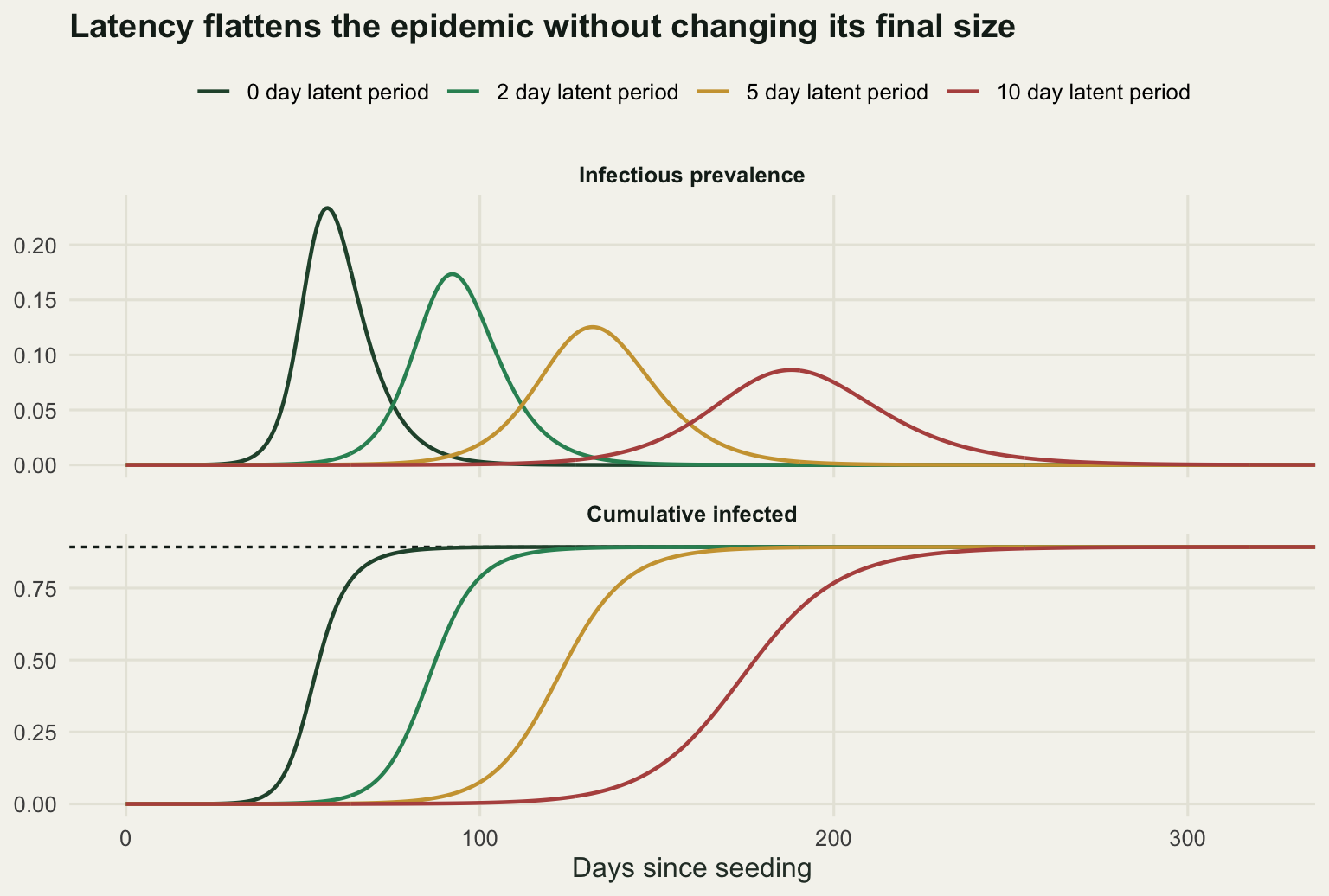

Figure 1: Infectious prevalence for four epidemics with the same reproduction number and the same infectious period, differing only in the mean latent period. The dashed line is the analytic final attack rate, which all four reach.

The exact relation between growth rate and reproduction number

Linearise the SEIR system about the disease free state. With \(S \approx 1\) the exposed and infectious classes obey a two by two linear system, and an exponential solution \(E, I \propto e^{rt}\) requires

\[(r + \sigma)(r + \gamma) = \sigma \beta.\]

Divide by \(\sigma\gamma\) and use \(R_0 = \beta/\gamma\) to get the form that matters for inference,

\[R_0 = \left(1 + \frac{r}{\sigma}\right)\left(1 + \frac{r}{\gamma}\right).\]

The second factor is the SIR answer. The first is the correction for latency, and it is larger than one whenever there is any latency at all. Setting \(\sigma\) to infinity kills it and returns \(R_0 = 1 + r/\gamma\).

There is a more general route that we need later, so it is worth setting up now. The Euler-Lotka condition says that at the exponential phase, one case must produce exactly one case per generation once future cases are discounted at rate \(r\). With constant infectiousness \(\beta\) during the infectious period, and independent latent and infectious durations,

\[1 = \beta\,\mathbb{E}\!\left[e^{-rT_{lat}}\right] \frac{1 - \mathbb{E}\!\left[e^{-rT_{inf}}\right]}{r}\]

so that \(R_0 = r / \left(\gamma \, \mathcal{L}_{lat}(r)\, (1 - \mathcal{L}_{inf}(r))\right)\), where \(\mathcal{L}\) is the Laplace transform of a duration. Exponential durations give \(\mathcal{L}(r) = \gamma/(\gamma + r)\) and reduce this to the product above. The code below implements the general version once, with Erlang durations of any stage count, and everything in the rest of the post is a special case of it.

lap_erlang <- function(r, mean_t, k) if (mean_t <= 0) 1 else (k / (mean_t * r + k))^k
r0_from_r <- function(r, lat_days, klat = 1, ninf = 1)
  r / (gam * lap_erlang(r, lat_days, klat) * (1 - lap_erlang(r, 1 / gam, ninf)))

check <- data.frame(latent_days = lat_set, r_fitted = tab$r_fitted,
                    r_closed_form = tab$r_closed_form)
check$r_gap_percent <- 100 * abs(check$r_fitted / check$r_closed_form - 1)
check$R0_from_fitted_r <- mapply(r0_from_r, check$r_fitted, check$latent_days)
check$R0_from_exact_r <- mapply(r0_from_r, check$r_closed_form, check$latent_days)
print(round(check, 6))

  latent_days r_fitted r_closed_form r_gap_percent R0_from_fitted_r
1           0 0.249976      0.250000      0.009665         2.499855
2           2 0.152561      0.152579      0.011833         2.499789
3           5 0.105805      0.105823      0.016435         2.499698
4          10 0.073477      0.073495      0.023486         2.499572
  R0_from_exact_r
1             2.5
2             2.5
3             2.5
4             2.5

print(signif(c(worst_r_gap_percent = max(check$r_gap_percent),
               worst_R0_gap_percent =
                 max(abs(100 * (check$R0_from_fitted_r / r0_true - 1)))), 4))

 worst_r_gap_percent worst_R0_gap_percent 
             0.02349              0.01714 

The closed form and the simulation agree to 0.02349 per cent in the growth rate at worst, and the gap grows with the latent period because a slower epidemic spends longer in the fitting window and therefore depletes slightly more susceptibles while it is being measured. Pushing the fitted growth rates back through the general inversion returns the true reproduction number to within 0.01714 per cent. That is a check of the algebra, not of the biology, and it is the only sense in which the relation is ever exact: it holds in the linear phase of a deterministic model with these exact duration distributions.

lat_grid <- seq(0, 14, by = 0.05)
r_grid <- sapply(lat_grid, r_exact)
gr_levels <- c("Growth rate r (per day)", "Doubling time (days)")
gr_line <- rbind(
  data.frame(latent = lat_grid, value = r_grid, quantity = gr_levels[1]),
  data.frame(latent = lat_grid, value = log(2) / r_grid, quantity = gr_levels[2]))
gr_pts <- rbind(
  data.frame(latent = tab$latent_days, value = tab$r_fitted, quantity = gr_levels[1]),
  data.frame(latent = tab$latent_days, value = tab$doubling_days,
             quantity = gr_levels[2]))
gr_line$quantity <- factor(gr_line$quantity, levels = gr_levels)
gr_pts$quantity <- factor(gr_pts$quantity, levels = gr_levels)

ggplot(gr_line, aes(latent, value)) +
  geom_line(colour = te_pal$forest, linewidth = 0.9) +
  geom_point(data = gr_pts, colour = te_pal$clay, size = 2.6, shape = 1, stroke = 1.2) +
  facet_wrap(~quantity, scales = "free_y") +
  labs(x = "Mean latent period (days)", y = NULL,
       title = "One reproduction number gives a whole family of growth rates") +
  theme_te() +
  theme(strip.text = element_text(colour = te_pal$ink, face = "bold"))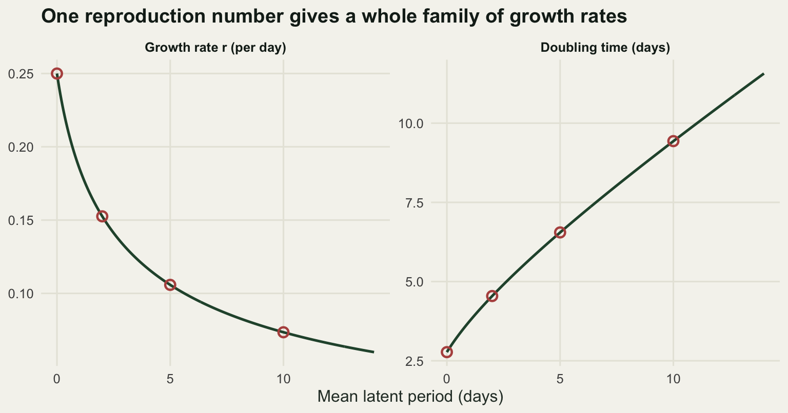

Figure 2: Early growth rate and doubling time against the mean latent period, at a fixed reproduction number of 2.5 and a fixed infectious period of six days. The line is the closed form root; the points are the growth rates fitted to the simulated epidemics.

Reading a real growth rate through the wrong model

Here is the practical version of the problem. An outbreak is under way. Someone fits an exponential curve to the first weeks of case reports and reports a growth rate. Someone else needs a reproduction number for a control target, opens a textbook, and finds \(R_0 = 1 + r/\gamma\). That formula is correct for SIR and wrong for every pathogen with a latent period, and it is wrong in one direction: too low.

The block below takes each simulated SEIR epidemic, which has a true reproduction number of 2.5 by construction, measures its growth rate, and inverts it both ways.

inv <- data.frame(latent_days = lat_set, r = tab$r_fitted,
                  sir_inversion = 1 + tab$r_fitted / gam,
                  seir_inversion = mapply(r0_from_r, tab$r_fitted, lat_set))
inv$underestimate_percent <- 100 * (1 - inv$sir_inversion / r0_true)
inv$recovery_error_percent <- 100 * abs(inv$seir_inversion / r0_true - 1)
print(round(inv, 5))

  latent_days       r sir_inversion seir_inversion underestimate_percent
1           0 0.24998       2.49986        2.49986               0.00580
2           2 0.15256       1.91537        2.49979              23.38530
3           5 0.10581       1.63483        2.49970              34.60677
4          10 0.07348       1.44086        2.49957              42.36545
  recovery_error_percent
1                0.00580
2                0.00842
3                0.01207
4                0.01714

print(round(c(control_target_from_sir_percent =
                100 * (1 - 1 / inv$sir_inversion[lat_set == 10]),
              control_target_true_percent = 100 * (1 - 1 / r0_true)), 4))

control_target_from_sir_percent     control_target_true_percent 
                        30.5972                         60.0000 

With a two day latent period the SIR inversion returns 1.91537 instead of 2.5, an underestimate of 23.3853 per cent. With five days it returns 1.63483, 34.60677 per cent low. With ten days it returns 1.44086, 42.36545 per cent low. The correct inversion returns 2.49979, 2.4997 and 2.49957, which is the truth to within 0.01714 per cent.

The size of the error is worth pausing on because of what gets decided with it. A reproduction number of 1.44086 says that removing 30.5972 per cent of transmission ends the outbreak. The true value of 2.5 says 60 per cent. Those are different interventions, different costs and, in a wildlife or livestock setting, a different culling or vaccination footprint. The failure is not in the estimate of \(r\), which was fine, but in the model used to translate it. And nothing in the data flags it: the epidemic curve does not carry a label saying which compartmental structure generated it.

Note also the direction. The SIR inversion is always the conservative one in the wrong sense. It makes the pathogen look easier to control than it is, because it implicitly assumes all of the generation interval is infectious time, so a slow epidemic must mean weak transmission rather than a long wait before transmission starts.

meth_levels <- c("SEIR inversion: (1 + r/gamma)(1 + r/sigma)",
                 "SIR inversion: 1 + r/gamma")
inv_line <- rbind(
  data.frame(latent = lat_grid, value = 1 + r_grid / gam, method = meth_levels[2]),
  data.frame(latent = lat_grid,
             value = mapply(r0_from_r, r_grid, lat_grid), method = meth_levels[1]))
inv_pts <- rbind(
  data.frame(latent = inv$latent_days, value = inv$sir_inversion,
             method = meth_levels[2]),
  data.frame(latent = inv$latent_days, value = inv$seir_inversion,
             method = meth_levels[1]))
inv_line$method <- factor(inv_line$method, levels = meth_levels)
inv_pts$method <- factor(inv_pts$method, levels = meth_levels)

ggplot(inv_line, aes(latent, value, colour = method)) +
  geom_hline(yintercept = r0_true, colour = te_pal$ink, linetype = "22",
             linewidth = 0.6) +
  geom_line(linewidth = 0.9) +
  geom_point(data = inv_pts, size = 2.6, shape = 1, stroke = 1.2) +
  scale_colour_manual(values = c(te_pal$forest, te_pal$clay), name = NULL) +
  guides(colour = guide_legend(nrow = 2)) +
  labs(x = "Mean latent period (days)", y = "Recovered R0",
       title = "The SIR formula loses more of R0 the longer the wait") +
  theme_te() +
  theme(legend.position = "top")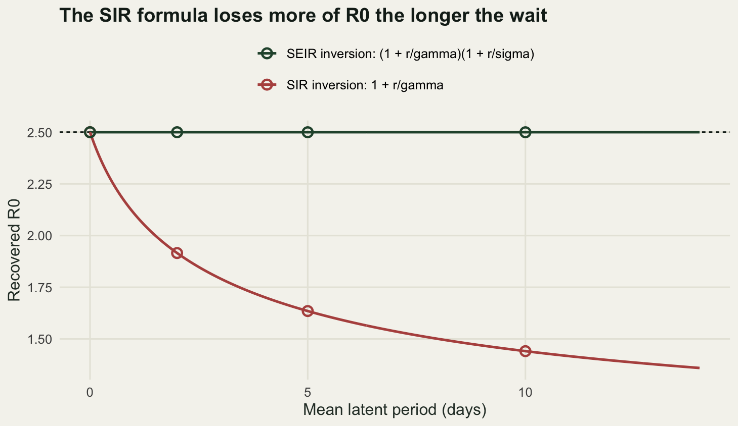

Figure 3: Reproduction number recovered from the measured growth rate of a SEIR epidemic whose true value is 2.5, using the SIR formula and using the SEIR formula. Points are the four simulated epidemics.

The mean is not the distribution

Everything above assumed the latent period is exponentially distributed, because that is what a single E compartment with a constant exit rate implies. An exponential latent period with a mean of five days has a standard deviation of five days, and its most likely value is zero: the commonest outcome under that model is becoming infectious almost immediately. No pathogen behaves like that.

The standard repair is a chain. Replace the single E box by \(k\) boxes in series, each with rate \(k\sigma\), so the total wait is a sum of \(k\) exponentials and follows an Erlang distribution with the same mean \(1/\sigma\) and standard deviation \(1/(\sigma\sqrt{k})\). As \(k\) grows the distribution tightens onto a fixed delay. The Laplace transform is \(\mathcal{L}(r) = (1 + r/(k\sigma))^{-k}\), so the inversion becomes

\[R_0 = \left(1 + \frac{r}{\gamma}\right)\left(1 + \frac{r}{k\sigma}\right)^{k} \longrightarrow \left(1 + \frac{r}{\gamma}\right)e^{rL}\]

with \(L = 1/\sigma\) the mean latent period. The question is how much this matters. Take one growth rate, the one measured from the five day exponential SEIR epidemic, and ask what reproduction number it implies under each shape at the same mean.

r_ref <- tab$r_fitted[lat_set == 5]
k_set <- c(1, 2, 4, 20)
erl <- data.frame(k = k_set,
                  latent_sd_days = 5 / sqrt(k_set),
                  R0_implied = sapply(k_set, function(k) r0_from_r(r_ref, 5, k)))
print(round(erl, 5))

   k latent_sd_days R0_implied
1  1        5.00000    2.49970
2  2        3.53553    2.61408
3  4        2.50000    2.68690
4 20        1.11803    2.75575

print(round(c(reference_growth_rate = r_ref,
              fixed_delay_limit = (1 + r_ref / gam) * exp(r_ref * 5),
              spread = max(erl$R0_implied) - min(erl$R0_implied),
              spread_percent = 100 * (max(erl$R0_implied) / min(erl$R0_implied) - 1)), 5))

reference_growth_rate     fixed_delay_limit                spread 
              0.10581               2.77476               0.25605 
       spread_percent 
             10.24326 

From a single growth rate of 0.10581 per day, one exposed stage gives 2.4997, two stages give 2.61408, four give 2.6869 and twenty give 2.75575, against a fixed delay limit of 2.77476. Every one of these assumes exactly the same mean latent period of five days and exactly the same measured epidemic curve. The spread is 0.25605 in absolute terms, or 10.24326 per cent. That is the honest size of the error you make by getting the shape wrong while getting the mean right, and it is smaller than the error from ignoring latency altogether, but it is not small.

The direction is consistent and it has a reason. A tighter latent period means fewer individuals become infectious unusually early, so to produce the same observed growth rate the pathogen must transmit harder. Any assumed distribution that is more variable than the truth will therefore understate \(R_0\), and the exponential is the most variable member of the Erlang family.

Because none of the above involved simulating a chain, it deserves a check against one. Run the four stage version at the same \(\beta\), \(\sigma\) and \(\gamma\), measure its growth rate, and invert it with the matching formula and with the exponential formula.

chain <- epi(5, m = 4)
r_chain <- as.numeric(fit_growth(chain)["r"])
print(round(c(chain_growth_rate = r_chain,
              recovered_with_k4 = r0_from_r(r_chain, 5, 4),
              recovered_assuming_exponential = r0_from_r(r_chain, 5, 1),
              underestimate_percent = 100 * (1 - r0_from_r(r_chain, 5, 1) / r0_true),
              attack_rate = 1 - min(chain$S)), 5))

             chain_growth_rate              recovered_with_k4 
                       0.09696                        2.49971 
recovered_assuming_exponential          underestimate_percent 
                       2.34867                        6.05311 
                   attack_rate 
                       0.89264 

print(signif(c(total_deviation = max(abs(chain$total - 1))), 4))

total_deviation 
      3.475e-14 

The four stage epidemic grows at 0.09696 per day, slower than the 0.10581 of the exponential version with the same mean, because a tight latent period means almost nobody short circuits it. Inverting with the four stage formula recovers 2.49971. Inverting with the exponential formula gives 2.34867, an underestimate of 6.05311 per cent. The attack rate is 0.89264 again, unchanged, because the final size relation still only knows \(R_0\).

dens_grid <- seq(0.001, 16, by = 0.02)
dens <- do.call(rbind, lapply(k_set, function(k)
  data.frame(x = dens_grid, y = dgamma(dens_grid, shape = k, rate = k / 5),
             stages = factor(paste(k, "stage"), levels = paste(k_set, "stage")))))
erl$stages <- factor(paste(erl$k, "stage"), levels = paste(k_set, "stage"))
delay_limit <- (1 + r_ref / gam) * exp(r_ref * 5)

p_dens <- ggplot(dens, aes(x, y, colour = stages)) +
  geom_line(linewidth = 0.9) +
  scale_colour_manual(values = c(te_pal$forest, te_pal$green, te_pal$gold,
                                 te_pal$clay), name = NULL) +
  coord_cartesian(ylim = c(0, 0.42)) +
  labs(x = "Latent period (days)", y = "Density",
       title = "The same mean allows four shapes") +
  theme_te() +
  theme(legend.position = "top",
        plot.title = element_text(face = "bold", colour = te_pal$ink,
                                  size = rel(0.9)))

p_r0 <- ggplot(erl, aes(k, R0_implied)) +
  geom_hline(yintercept = delay_limit, colour = te_pal$ink, linetype = "22",
             linewidth = 0.6) +
  geom_hline(yintercept = r0_true, colour = te_pal$sage, linewidth = 0.8) +
  geom_line(colour = te_pal$forest, linewidth = 0.8) +
  geom_point(aes(colour = stages), size = 3.2) +
  scale_colour_manual(values = c(te_pal$forest, te_pal$green, te_pal$gold,
                                 te_pal$clay), guide = "none") +
  scale_x_log10(breaks = k_set) +
  labs(x = "Number of exposed stages k", y = "Recovered R0",
       title = "One growth rate gives four answers") +
  theme_te() +
  theme(plot.title = element_text(face = "bold", colour = te_pal$ink,
                                  size = rel(0.9)))

grid.newpage()
pushViewport(viewport(layout = grid.layout(1, 2)))
print(p_dens, vp = viewport(layout.pos.row = 1, layout.pos.col = 1))
print(p_r0, vp = viewport(layout.pos.row = 1, layout.pos.col = 2))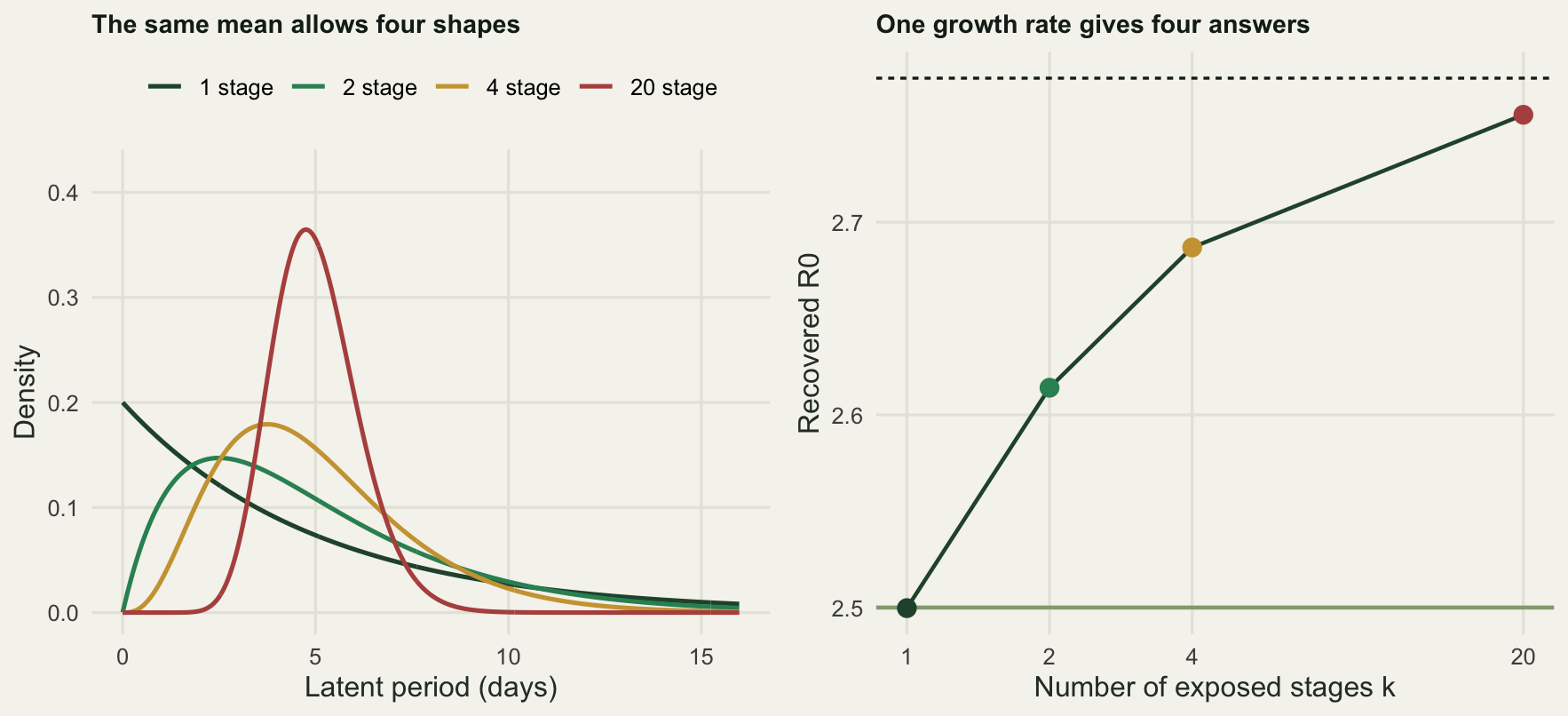

Figure 4: Latent period distributions with the same five day mean but different stage counts, and the reproduction number each one implies from a single measured growth rate.

The honest limit: the infectious period has a shape too

Every correction so far fixed the latent period and left the infectious period alone. The infectious period in all of these models is exponential, with a mean of six days, which carries exactly the same defect: it says the commonest duration of infectiousness is close to zero. Real shedding periods are far tighter than that.

The general inversion already handles it. Give the infectious period \(n\) stages of rate \(n\gamma\) and its Laplace transform is \((1 + r/(n\gamma))^{-n}\), so

\[R_0 = \frac{r}{\gamma \, \mathcal{L}_{lat}(r) \, \left(1 - (1 + r/(n\gamma))^{-n}\right)}.\]

The measurement below is the one that matters. Simulate an epidemic with an exponential five day latent period and a four stage infectious period of the same six day mean, measure its growth rate, and invert it two ways: with the correct four stage infectious formula, and with the exponential one that almost every published inversion uses.

gam_chain <- epi(5, m = 1, n = 4)
r_gc <- as.numeric(fit_growth(gam_chain)["r"])
print(round(c(growth_rate = r_gc,
              recovered_correctly = r0_from_r(r_gc, 5, 1, 4),
              recovered_assuming_exponential = r0_from_r(r_gc, 5, 1, 1),
              overestimate_percent = 100 * (r0_from_r(r_gc, 5, 1, 1) / r0_true - 1),
              infectious_sd_days = inf_days / sqrt(4),
              peak_prevalence = max(gam_chain$prev),
              peak_day = gam_chain$t[which.max(gam_chain$prev)],
              attack_rate = 1 - min(gam_chain$S)), 5))

                   growth_rate            recovered_correctly 
                       0.12827                        2.49976 
recovered_assuming_exponential           overestimate_percent 
                       2.90461                       16.18438 
            infectious_sd_days                peak_prevalence 
                       3.00000                        0.15819 
                      peak_day                    attack_rate 
                     108.50000                        0.89264 

This epidemic grows at 0.12827 per day, faster than the 0.10581 of the fully exponential SEIR with the same two means, because a tight infectious period stops individuals recovering in the first day and so keeps early transmission going. The correct inversion recovers 2.49976. The inversion that gets the latent period exactly right and the infectious period wrong returns 2.90461, which is 16.18438 per cent too high.

That result went the opposite way from what I expected before running it, and it is the most useful thing in the post. The latent period corrections all pushed the estimate up, and getting the latent shape wrong pushed it down by 6.05311 per cent. Here the infectious shape error pushes it up by 16.18438 per cent, and it is more than twice as large. The two errors partly cancel in a real analysis, which is worse than either alone, because it means an inversion with two wrong assumptions can look better than an inversion with one, and the analyst has no way to tell which situation they are in.

The deeper limit is that all of this is a statement about generation intervals and nothing else. The growth rate constrains one functional of the generation interval distribution, its Laplace transform at \(r\), and the reproduction number is what you get by dividing that out. An epidemic curve does not contain the generation interval distribution. It has to come from contact tracing, from challenge experiments, or from shedding studies, and in wildlife disease it usually comes from none of these. When it is unavailable, the correct output is not a reproduction number but a range of them, computed across the shapes that the biology does not exclude, and the spread of 10.24326 per cent measured above for latent shape alone is the floor of that range rather than the whole of it.

Two further limits are worth stating without measuring them, because this post’s machinery cannot see them. Everything here is deterministic, so it says nothing about the stochastic early phase where most introductions die out. And the whole exercise assumes the population is well mixed, which for a territorial mammal or a colonial breeder is the assumption most likely to be false.

Where to go next

The inversion in this post takes a growth rate as given. Measuring that growth rate from real incidence data, which arrive as noisy counts with reporting delays rather than as a smooth curve, is a separate problem with its own failure modes, and Estimating R0 from incidence data works through it. The natural extension in the other direction is what happens when susceptibles are replenished by births, which turns the single epidemic here into a recurrent one and brings the latent period back as a determinant of the interepidemic period.

References

Kermack WO, McKendrick AG 1927 Proceedings of the Royal Society A 115(772):700-721 (10.1098/rspa.1927.0118)

Wearing HJ, Rohani P, Keeling MJ 2005 PLoS Medicine 2(7):e174 (10.1371/journal.pmed.0020174)

Wallinga J, Lipsitch M 2007 Proceedings of the Royal Society B 274(1609):599-604 (10.1098/rspb.2006.3754)

Keeling MJ, Rohani P 2008 Modeling Infectious Diseases in Humans and Animals. Princeton University Press, ISBN 978-0-691-11617-4

Anderson RM, May RM 1991 Infectious Diseases of Humans: Dynamics and Control. Oxford University Press, ISBN 978-0-19-854040-3

Related tutorials

• Estimating R0 from incidence data
• Seasonality and recurrent epidemics
• Checking an epidemic estimate
• The SIR epidemic model