The SIR epidemic model

The SIR model in R: building an epidemic from susceptible, infected and recovered compartments, and why the reproduction number decides whether it spreads.

An epidemic in a wildlife population, or any population, is a flow between three pools: hosts that can still catch the disease, hosts that have it and are spreading it, and hosts that have recovered (or died) and are no longer in play. The SIR model, from Kermack and McKendrick 1927 Proceedings of the Royal Society A 115(772):700-721, tracks those three pools and asks the question every disease ecologist starts with: given how fast the pathogen spreads and how fast hosts recover, will it take off or fizzle out?

Three compartments and two rates

Write the population as fractions: S susceptible, I infected, R recovered. Two processes move hosts between them. Infection moves a susceptible to infected at a rate set by how often susceptibles and infecteds meet, the transmission rate times the product of the two fractions. Recovery moves an infected to recovered at a constant per-capita rate. That is the whole model, integrated forward in time.

sir_step <- function(S, I, R, beta, gamma, dt) {
  dS <- -beta*S*I                 # susceptibles become infected on contact
  dI <-  beta*S*I - gamma*I       # infecteds arrive, and recover at rate gamma
  dR <-  gamma*I                  # recovered accumulate
  c(S + dS*dt, I + dI*dt, R + dR*dt)
}
beta <- 0.4; gamma <- 0.1        # transmission rate and recovery rate (per day)
state <- c(1 - 1e-3, 1e-3, 0)    # start almost all susceptible, a seed of infection
for (k in 1:20000) state <- sir_step(state[1], state[2], state[3], beta, gamma, 0.01)
round(state, 3)                  # S, I, R at the end

[1] 0.02 0.00 0.98

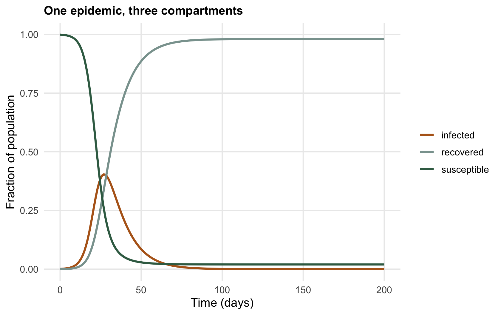
Starting from a nearly healthy population with a seed of infection, the epidemic runs its course and burns out: infecteds return to zero, but not before a large share of the population has passed through. The three curves together tell the story, susceptibles draining, infecteds cresting and falling, recovered filling up.

dl <- rbind(data.frame(t = ep$t, frac = ep$S, comp = "susceptible"),
            data.frame(t = ep$t, frac = ep$I, comp = "infected"),
            data.frame(t = ep$t, frac = ep$R, comp = "recovered"))
ggplot(dl, aes(t, frac, colour = comp)) +
  geom_line(linewidth = 1) +
  scale_colour_manual(values = c("susceptible" = col_S, "infected" = col_I, "recovered" = col_R)) +
  labs(x = "Time (days)", y = "Fraction of population", colour = NULL,
       title = "One epidemic, three compartments")

Figure 1: The SIR epidemic. Susceptibles (green) fall as the infection spreads, the infected fraction (ochre) rises to a peak and declines, and the recovered (grey) accumulate. The epidemic ends when susceptibles run too low to sustain it.

The number that decides everything

Whether the pathogen spreads at all comes down to a single quantity. Each infected host, over its infectious period, passes the disease to some average number of others; when the population is fully susceptible, that number is the basic reproduction number. In the SIR model it is the transmission rate divided by the recovery rate, because an infection lasts on average one over the recovery rate and spreads at the transmission rate throughout.

c(R0 = beta/gamma, mean_infectious_period_days = 1/gamma)

                         R0 mean_infectious_period_days 
                          4                          10 

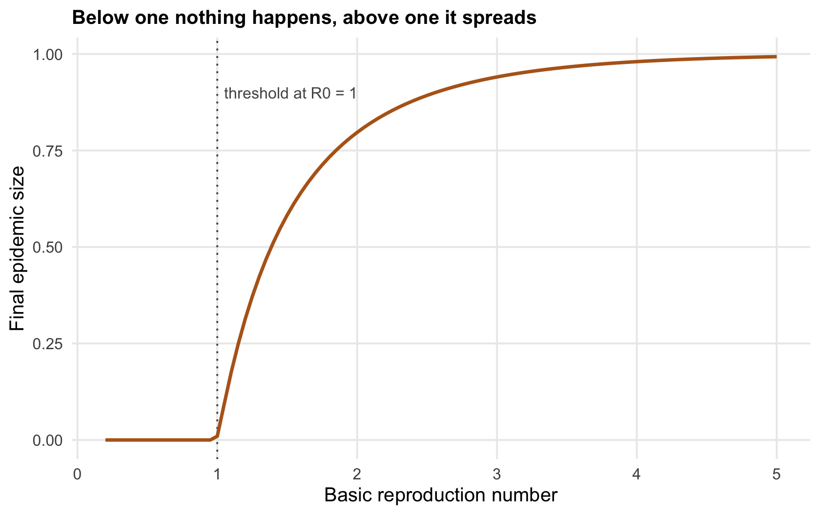
Here the basic reproduction number is 4: each case seeds four more at the outset. That is what drives the epidemic, and it sets its scale. The infected fraction peaks at 0.40 of the population around day 27, and by the end 0.98 of the population has been infected: the final epidemic size, the total that ever leaves the susceptible pool. That final size is not something you have to simulate to find; it is the solution of a short self-referential equation set only by the reproduction number.

R0g <- seq(0.2, 5, 0.05)
dg <- data.frame(R0 = R0g, size = sapply(R0g, fs_eqn))
ggplot(dg, aes(R0, size)) +
  geom_vline(xintercept = 1, colour = col_ref, linetype = "dotted") +
  geom_line(colour = col_I, linewidth = 1) +
  annotate("text", x = 1.05, y = 0.9, label = "threshold at R0 = 1", hjust = 0, colour = col_ref, size = 3.4) +
  labs(x = "Basic reproduction number", y = "Final epidemic size",
       title = "Below one nothing happens, above one it spreads")

Figure 2: The final epidemic size against the basic reproduction number. Below one the pathogen cannot spread and no epidemic occurs; above one the fraction eventually infected climbs steeply toward the whole population.

What the model gives, and what it assumes

The SIR model is the foundation of disease ecology because it turns a messy process into two rates and one threshold, and from those it predicts whether a pathogen invades, how large the outbreak is, and when it peaks. Those predictions are the levers management pulls: lower the transmission rate or shorten the infectious period and you push the reproduction number down toward the threshold. But the simplicity comes from strong assumptions, that hosts mix at random, that the population is closed over the outbreak, that everyone is equally susceptible and equally infectious, and each of those is a place the model can mislead. The threshold itself, and the herd immunity it implies, is the next post; what happens when births refill the susceptible pool is endemic disease; and the assumptions that most often break are the checking post.

Related tutorials

• R0 and herd immunity
• Host density and endemic disease
• Checking an epidemic model
• The Levins metapopulation model

References

• Kermack WO, McKendrick AG 1927. Proceedings of the Royal Society A 115(772):700-721 (10.1098/rspa.1927.0118).
• Anderson RM, May RM 1979. Nature 280(5721):361-367 (10.1038/280361a0).