---
title: "Host density and endemic disease"
description: "Endemic disease in R: why density-dependent transmission gives a host-density threshold for invasion, and how a pathogen settles to an endemic prevalence."
date: "2026-07-05 11:00"
categories: [ecology tutorial, R, disease ecology, population models, theoretical ecology]
image: thumbnail.png
image-alt: "The reproduction number rising with host density and crossing one at a threshold density below which the pathogen cannot invade."
date-modified: "2026-09-27"
---
*Corrected 27 September 2026: the text described the climb to the endemic level as fastest at the start; it now says, as the figure shows, that the climb is S-shaped, slow while infections are rare and fastest at intermediate prevalence.*
```{r setup}
#| code-fold: true
#| code-summary: "Setup: packages, colours and plot theme"
#| results: hide
#| message: false
#| warning: false
knitr::opts_chunk$set(echo = TRUE, message = FALSE, warning = FALSE,
                      dev = "png", dpi = 120, fig.path = "figures/",
                      fig.width = 7, fig.height = 4.4)
library(ggplot2)
theme_te <- theme_minimal(base_size = 12) +
  theme(panel.background = element_rect(fill = "#f5f4ee", colour = NA),
        plot.background  = element_rect(fill = "#f5f4ee", colour = NA),
        panel.grid.minor = element_blank(),
        plot.title = element_text(face = "bold", size = 12))
theme_set(theme_te)
col_a <- "#3a6b52"; col_b <- "#b5651d"; col_ref <- "#555555"

b <- 0.002; gamma <- 0.1              # transmission per contact, recovery rate
N_T <- gamma/b                        # host-density threshold
R0_dens <- function(N) b*N/gamma
sis <- function(R0, I0 = 1e-3, Tn = 300, dt = 0.05) {
  I <- I0; out <- data.frame(t = 0, I = I)
  for (k in 1:(Tn/dt)) { I <- I + (R0*gamma*(1 - I)*I - gamma*I)*dt
    if (k %% round(1/dt) == 0) out <- rbind(out, data.frame(t = k*dt, I = I)) }
  out
}
endemic <- function(R0) max(0, 1 - 1/R0)
```
The [SIR model](../the-sir-epidemic-model/) treats one closed outbreak, but most wildlife diseases are not one-off events; they smoulder, persist, and flare again as new susceptibles are born. Whether a pathogen can establish and persist at all often depends on something the basic model hides inside its transmission term: how many hosts there are. For many diseases there is a threshold host density below which the pathogen simply cannot invade, and that single fact shapes how disease regulates wildlife and whether culling can ever clear it.
## Transmission that scales with density
When infection spreads through direct contact, the rate at which a susceptible meets an infected host rises with how crowded the population is. In a denser population there are more contacts per unit time, so the transmission term scales with host density rather than being fixed. That makes the reproduction number itself depend on density: it is the per-contact transmission times host density, divided by the recovery rate.
```{r threshold}
b <- 0.002; gamma <- 0.1             # b = transmission per host per contact
R0_dens <- function(N) b*N/gamma     # reproduction number rises with density
c(N30 = R0_dens(30), N50 = R0_dens(50), N80 = R0_dens(80))
```
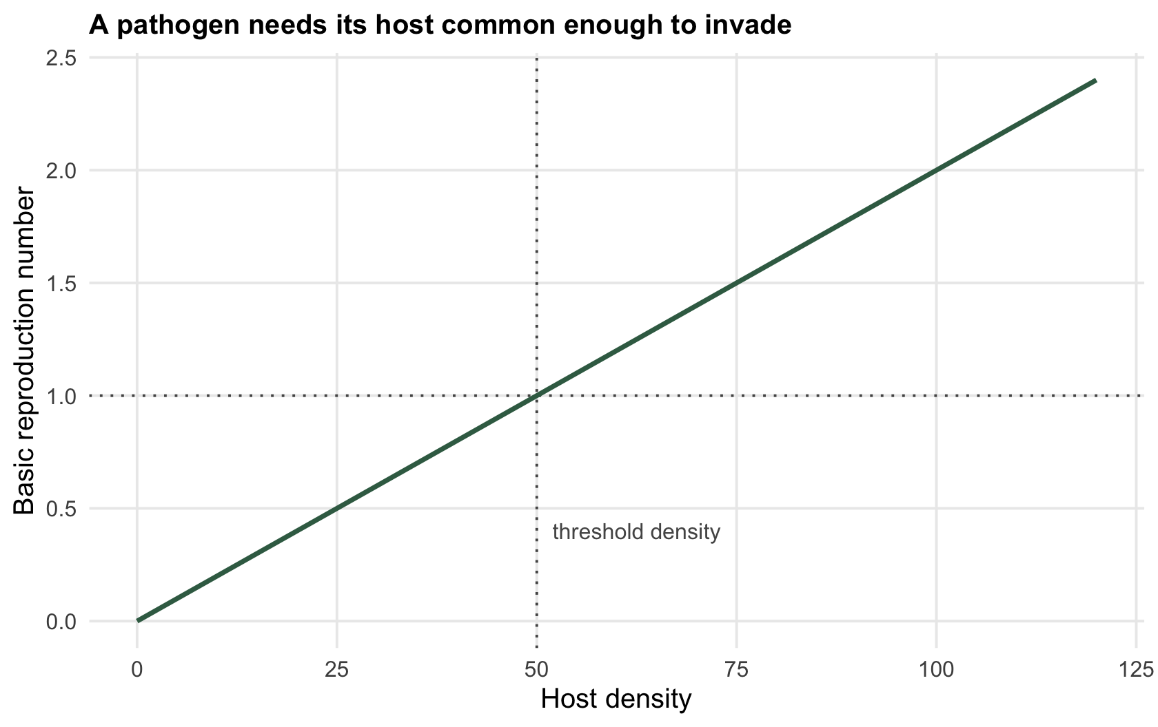
At low density the reproduction number sits below one and the pathogen cannot spread; at high density it clears one and an epidemic becomes possible. The density where it crosses one is the threshold host density, the transmission-and-recovery combination that makes each case exactly replace itself.
```{r nt}
N_T <- gamma/b                       # host-density threshold: R0 = 1
N_T
```
The threshold density here is `r sprintf("%.0f", N_T)` hosts. Below it the pathogen fades out no matter how it is introduced; above it the disease can invade and the reproduction number keeps climbing with density. This is the classic result that gives disease a role in ecology it would not otherwise have: a pathogen with density-dependent transmission can only persist where its host is common enough, so it tends to knock the host back toward that threshold and hold it there rather than driving it extinct.
```{r fig-threshold}
#| fig-cap: "The reproduction number against host density under density-dependent transmission. Below the threshold density (dotted) the pathogen cannot invade; above it the disease spreads and the reproduction number keeps rising."
#| fig-alt: "A rising straight line of reproduction number against host density crossing a horizontal line at one, at the threshold density marked with a dotted vertical line."
Ng <- seq(0, 120, 1)
dg <- data.frame(N = Ng, R0 = R0_dens(Ng))
ggplot(dg, aes(N, R0)) +
  geom_hline(yintercept = 1, colour = col_ref, linetype = "dotted") +
  geom_vline(xintercept = N_T, colour = col_ref, linetype = "dotted") +
  geom_line(colour = col_a, linewidth = 1) +
  annotate("text", x = N_T + 2, y = 0.4, label = "threshold density", hjust = 0, colour = col_ref, size = 3.4) +
  labs(x = "Host density", y = "Basic reproduction number",
       title = "A pathogen needs its host common enough to invade")
```
## Settling to an endemic level
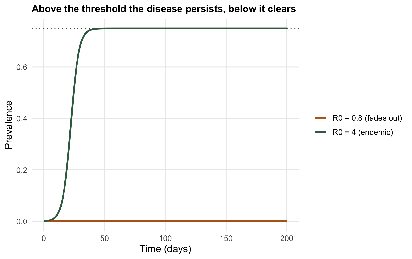
Above the threshold, a pathogen that hosts can catch more than once does not burn out; it settles to a steady prevalence where new infections exactly balance recoveries. In the simplest such model, where recovered hosts become susceptible again, that endemic prevalence is one minus one over the reproduction number, the same expression as the herd immunity threshold, now describing where the disease sits rather than where it stops.
```{r sis}
sis <- function(R0, I0 = 1e-3, Tn = 300, dt = 0.05) {
  I <- I0
  for (k in 1:(Tn/dt)) I <- I + (R0*gamma*(1 - I)*I - gamma*I)*dt   # susceptibles = 1 - I
  I
}
c(R0_4_endemic = sis(4), analytic = 1 - 1/4, R0_0.8 = sis(0.8))
```
With a reproduction number of `r sprintf("%.0f", 4)` the disease settles at a prevalence of `r sprintf("%.2f", endemic(4))`, exactly one minus one over the reproduction number, and stays there indefinitely: an endemic infection. Drop the reproduction number below one, whether by thinning the host population below the threshold density or by any other route, and the prevalence falls to zero and the pathogen is gone. The endemic level is reached by an S-shaped climb: slow while infections are rare, fastest at intermediate prevalence, and slowing as the prevalence nears its ceiling.
```{r fig-endemic}
#| fig-cap: "Prevalence over time for a persistent infection. Above the threshold (green) it climbs to a steady endemic level, one minus one over the reproduction number; below it (ochre) the pathogen dies out."
#| fig-alt: "Two prevalence curves over time; one rises and levels off at a positive endemic value, the other decays to zero."
traj <- function(R0) { I <- 1e-3; d <- data.frame(t = 0, I = I)
  for (k in 1:4000) { I <- I + (R0*gamma*(1 - I)*I - gamma*I)*0.05; if (k %% 20 == 0) d <- rbind(d, data.frame(t = k*0.05, I = I)) }; d }
dd <- rbind(cbind(traj(4), case = "R0 = 4 (endemic)"), cbind(traj(0.8), case = "R0 = 0.8 (fades out)"))
ggplot(dd, aes(t, I, colour = case)) +
  geom_hline(yintercept = endemic(4), colour = col_ref, linetype = "dotted") +
  geom_line(linewidth = 1) +
  scale_colour_manual(values = c("R0 = 4 (endemic)" = col_a, "R0 = 0.8 (fades out)" = col_b)) +
  labs(x = "Time (days)", y = "Prevalence", colour = NULL,
       title = "Above the threshold the disease persists, below it clears")
```
## The threshold is a modelling choice, not a fact
The host-density threshold is one of the most useful ideas in disease ecology and one of the most fragile, because it depends entirely on transmission scaling with density. That assumption is right for many directly transmitted diseases but wrong for others: sexually transmitted and some vector-borne pathogens spread at a rate set by the *frequency* of infecteds, not their density, and those have no host-density threshold at all and cannot be controlled by thinning the population. Which form transmission takes is the single most consequential choice in a wildlife disease model: it decides whether culling helps or is useless, and it is rarely settled by the data. That choice, and the other assumptions that quietly set the answer, are the subject of the [checking post](../checking-an-epidemic-model/).
## References
- Anderson RM, May RM 1979. Nature 280(5721):361-367 (10.1038/280361a0).
- Lloyd-Smith JO, Cross PC, Briggs CJ, Daugherty M, Getz WM et al. 2005. Trends in Ecology and Evolution 20(9):511-519 (10.1016/j.tree.2005.07.004).
## Related tutorials
- [The SIR epidemic model](../the-sir-epidemic-model/)
- [Density or frequency transmission in enclosures](../density-or-frequency-dependent-transmission/)
- [Fertility control versus culling in R](../fertility-control-versus-culling/)
- [Force of infection from age prevalence](../force-of-infection-from-age-prevalence/)