library(ggplot2)
library(patchwork)

te_paper  <- "#f5f4ee"
te_ink    <- "#16241d"
te_body   <- "#2c3a31"
te_forest <- "#275139"
te_rust   <- "#b5534e"
te_gold   <- "#c9b458"
te_line   <- "#dad9ca"

theme_datasheet <- function() {
  theme_minimal(base_size = 12) +
    theme(plot.background  = element_rect(fill = te_paper, colour = NA),
          panel.background = element_rect(fill = te_paper, colour = NA),
          panel.grid.major = element_line(colour = te_line, linewidth = 0.3),
          panel.grid.minor = element_blank(),
          text             = element_text(colour = te_body),
          plot.title       = element_text(colour = te_ink, face = "bold"),
          plot.subtitle    = element_text(colour = te_body),
          axis.text        = element_text(colour = te_body))
}Density or frequency transmission in enclosures
R
disease ecology
epidemiology
GLM
experimental design
simulation
ecology tutorial
Enclosure trials tell density- from frequency-dependent transmission apart only over a wide range of group sizes. A cloglog GLM, its interval and repairs in R.
Twelve outdoor enclosures of equal area, stocked with 5, 10, 20 or 40 voles, three enclosures at each group size. One animal in each enclosure is inoculated with a directly transmitted virus, and every animal is checked daily until the outbreak has run its course. The question the experiment exists to answer is how transmission scales with the number of hosts. If contacts rise with crowding, transmission is density dependent, the reproduction number grows with host numbers, and a cull can push it below one. If each animal keeps roughly the same number of contacts however many neighbours it has, transmission is frequency dependent, and thinning the population does nothing to the reproduction number.
This site has already made the management half of that argument. Checking an epidemic model draws the reproduction number against host density under both forms and concludes that the form is almost never identifiable from a single epidemic curve, so it has to be argued from biology. Host density and endemic disease calls the density threshold a modelling choice, not a fact. Neither post estimates anything. McCallum, Barlow and Hone 2001 made the design argument this post runs on: the two forms can be told apart only by watching transmission across a range of host densities, and Begon and colleagues 2002 fixed the terms, pointing out that density and number are different things once area varies. So the comparison of forms is known; what the post does is price the design. How wide a range of group sizes is needed, what happens to the interval when enclosures differ, and which enclosure-level repair holds its level with twelve enclosures.
The fitting tool is the one used in force of infection from age prevalence: a binomial GLM with a complementary log-log link and an offset. There the offset was log age. Here it is the log of the number of infectious animals on the day, and the coefficient of log group size is the transmission exponent.
One chain binomial, three models
Each day, each susceptible animal escapes infection with probability exp(-beta I N^-q), where I is the number of infectious animals and N the group size. An exponent q of zero is density dependence at fixed area; q of one is frequency dependence. Infectious animals recover with a fixed daily probability. The complementary log-log of the daily infection probability is then log beta + log I - q log N, which is a GLM with log I as offset: fix the coefficient of log N at zero for the density model, at minus one for the frequency model, or estimate it.
The daily rate is calibrated so that the two forms agree for a group of ten in unit area: a per-pair daily hazard of 0.03 either way, with a recovery probability of 0.1 per day. Every enclosure gets its own transmission rate, drawn as a lognormal around that common value; the spread is a design constant, zero for now. The simulator keeps each enclosure’s log draw beside its day records, which no real experiment would know, so that one check further down can use it. Groups can also be held at a fixed size in enclosures of different area, in which case the per-pair hazard is beta N^-q A^(q-1): area enters with exponent minus one under density dependence and not at all under frequency dependence.
gam_rec <- 0.1     # daily recovery probability
b_ref   <- 0.03    # per-pair daily hazard for ten animals in unit area
n_ref   <- 10
max_day <- 150

sim_experiments <- function(n_exp, sizes, reps, q, sd_log, area = 1) {
  n_arm <- max(length(sizes), length(area))
  arm_n <- rep(sizes, length.out = n_arm); arm_a <- rep(area, length.out = n_arm)
  arm <- rep(seq_len(n_arm), each = reps); n_encl <- length(arm)
  N <- rep(arm_n[arm], n_exp); A <- rep(arm_a[arm], n_exp)
  exper <- rep(seq_len(n_exp), each = n_encl); encl <- rep(seq_len(n_encl), n_exp)
  stratum <- rep(arm, n_exp)
  log_draw <- rnorm(length(N), 0, sd_log)
  beta_encl <- b_ref * n_ref^q * exp(log_draw)
  S <- N - 1; I <- rep(1, length(N)); days <- vector("list", max_day)
  for (day in seq_len(max_day)) {
    live <- which(I > 0 & S > 0)
    if (length(live) == 0) break
    p_inf <- 1 - exp(-beta_encl[live] * I[live] * N[live]^(-q) * A[live]^(q - 1))
    new <- rbinom(length(live), S[live], p_inf)
    rec <- rbinom(length(live), I[live], gam_rec)
    days[[day]] <- cbind(exper[live], encl[live], stratum[live], S[live], I[live],
                         N[live], A[live], new, log_draw[live])
    S[live] <- S[live] - new; I[live] <- I[live] + new - rec
  }
  out <- do.call(rbind, days)
  colnames(out) <- c("exper", "encl", "stratum", "S", "I", "N", "A", "new", "log_draw")
  out <- as.data.frame(out[order(out[, "exper"], out[, "encl"]), ])
  attr(out, "n_encl") <- n_encl
  out
}
r0_approx <- function(N, q) b_ref * n_ref^q * N^(-q) * (N - 1) / gam_rec
With these constants the rough reproduction number, hazard times susceptibles times mean infectious period, runs from 1.2 in a group of five to 11.7 in a group of forty under density dependence, and from 2.4 to 2.9 under frequency dependence.
Thousands of experiments means tens of thousands of GLM fits, so the fitting is done once for all experiments at a time: iteratively reweighted least squares for the complementary log-log binomial, with every experiment as a group and step halving when the likelihood falls. The function returns what glm() returns for the transmission exponent: estimate, model standard error, and the log-likelihoods of the density and frequency models. Both of those models have one free parameter, so comparing their AIC is comparing their likelihoods. It also returns two quantities used later: the Pearson dispersion of the day records and a cluster sandwich standard error that sums the score over enclosures.
irls_cloglog <- function(new, S, x, off, grp, mult = 1, a0 = NULL, b0 = 0,
                         n_it = 100, tol = 1e-8) {
  n_grp <- max(grp); w0 <- S * mult; has_x <- !is.null(x)
  if (!has_x) x <- rep(0, length(new))
  if (is.null(a0)) a0 <- log((rowsum(mult * new, grp)[, 1] + 0.5) /
                             rowsum(w0 * exp(off), grp)[, 1])
  a <- rep_len(a0, n_grp); b <- if (has_x) rep_len(b0, n_grp) else rep(0, n_grp)
  ll_rows <- function(aa, bb, ix) {
    ee <- exp(aa + bb * x[ix] + off[ix])
    mult_i <- if (length(mult) == 1) mult else mult[ix]
    mult_i * (lchoose(S[ix], new[ix]) +
              ifelse(new[ix] > 0, new[ix] * log(-expm1(-ee)), 0) - (S[ix] - new[ix]) * ee)
  }
  ll_grp <- function(aa, bb, ix, g) rowsum(ll_rows(aa[g], bb[g], ix), g)[, 1]
  active <- rep(TRUE, n_grp)
  for (it in seq_len(n_it)) {
    ix <- which(active[grp]); if (length(ix) == 0) break
    g <- grp[ix]; ids <- sort(unique(g))
    lin <- a[g] + b[g] * x[ix]
    eta <- lin + off[ix]; eta[eta < -30] <- -30; eta[eta > 3] <- 3
    ee <- exp(eta); mu <- -expm1(-ee); mu[mu > 1 - 1e-12] <- 1 - 1e-12
    dmu <- ee * exp(-ee); wt <- w0[ix] * dmu^2 / (mu * (1 - mu))
    z <- lin + (new[ix] / S[ix] - mu) / dmu; xx <- x[ix]
    s0 <- rowsum(wt, g)[, 1]; sz <- rowsum(wt * z, g)[, 1]
    a_new <- a; b_new <- b
    if (has_x) {
      s1 <- rowsum(wt * xx, g)[, 1]; s2 <- rowsum(wt * xx^2, g)[, 1]
      s1z <- rowsum(wt * xx * z, g)[, 1]; dt <- s0 * s2 - s1^2
      a_new[ids] <- (s2 * sz - s1 * s1z) / dt; b_new[ids] <- (s0 * s1z - s1 * sz) / dt
    } else a_new[ids] <- sz / s0
    ll_old <- rep(-Inf, n_grp); ll_old[ids] <- ll_grp(a, b, ix, g)
    ll_new <- rep(-Inf, n_grp); ll_new[ids] <- ll_grp(a_new, b_new, ix, g)
    for (h in 1:30) {
      worse <- ids[!(is.finite(ll_new[ids]) & ll_new[ids] >= ll_old[ids] - 1e-10)]
      if (length(worse) == 0) break
      a_new[worse] <- (a[worse] + a_new[worse]) / 2
      b_new[worse] <- (b[worse] + b_new[worse]) / 2
      jx <- which(grp %in% worse)
      ll_new[worse] <- ll_grp(a_new, b_new, jx, grp[jx])
    }
    step <- pmax(abs(a_new - a), abs(b_new - b))
    a <- a_new; b <- b_new
    active[ids] <- step[ids] > tol
  }
  eta <- a[grp] + b[grp] * x + off; ee <- exp(eta); mu <- -expm1(-ee)
  mu[mu > 1 - 1e-12] <- 1 - 1e-12; mu[mu < 1e-300] <- 1e-300
  dmu <- ee * exp(-ee); wt <- w0 * dmu^2 / (mu * (1 - mu))
  info <- if (has_x) cbind(rowsum(wt, grp)[, 1], rowsum(wt * x, grp)[, 1],
                           rowsum(wt * x^2, grp)[, 1]) else rowsum(wt, grp)[, 1]
  list(a = a, b = b, mu = mu, dmu = dmu, info = info,
       loglik = rowsum(ll_rows(a[grp], b[grp], seq_along(new)), grp)[, 1])
}

fit_day_level <- function(dat, covariate = "N") {
  grp <- dat$exper; lx <- log(dat[[covariate]]); off_i <- log(dat$I)
  by_n <- covariate == "N"
  f_dd <- irls_cloglog(dat$new, dat$S, NULL, if (by_n) off_i else off_i - lx, grp)
  f_fd <- irls_cloglog(dat$new, dat$S, NULL, if (by_n) off_i - lx else off_i, grp)
  f_q  <- irls_cloglog(dat$new, dat$S, lx, off_i, grp)
  inf <- f_q$info; dt <- inf[, 1] * inf[, 3] - inf[, 2]^2
  mu <- f_q$mu; n_row <- tabulate(grp)
  pearson <- rowsum((dat$new - dat$S * mu)^2 / (dat$S * mu * (1 - mu)), grp)[, 1]
  score <- (dat$new - dat$S * mu) * f_q$dmu / (mu * (1 - mu))
  n_encl <- attr(dat, "n_encl"); clus <- (grp - 1) * n_encl + dat$encl
  u0 <- rowsum(score, clus)[, 1]; u1 <- rowsum(score * lx, clus)[, 1]
  clus_grp <- (as.numeric(names(u0)) - 1) %/% n_encl + 1
  m00 <- rowsum(u0^2, clus_grp)[, 1]; m01 <- rowsum(u0 * u1, clus_grp)[, 1]
  m11 <- rowsum(u1^2, clus_grp)[, 1]; n_cl <- tabulate(clus_grp)
  c0 <- -inf[, 2] / dt; c1 <- inf[, 1] / dt
  se <- sqrt(inf[, 1] / pmax(dt, 0)); se[!is.finite(se)] <- Inf
  se_cr <- sqrt(pmax(0, c0^2 * m00 + 2 * c0 * c1 * m01 + c1^2 * m11) * n_cl / (n_cl - 1))
  se_cr[!is.finite(se_cr)] <- Inf
  data.frame(pick_dd = f_dd$loglik > f_fd$loglik,
             q_hat = if (by_n) -f_q$b else f_q$b + 1, se = se,
             dispersion = pearson / (n_row - 2), n_row = n_row,
             se_cr = se_cr, n_cl = n_cl, a_hat = f_q$a, b_hat = f_q$b)
}
A shortcut of this kind is a claim to check, not to assert. Ten experiments fitted both ways:
set.seed(4101)
chk_dat <- sim_experiments(10, c(5, 10, 20, 40), 3, 0.5, 0.6)
chk_fit <- fit_day_level(chk_dat)
chk_ref <- t(sapply(1:10, function(e) {
  s_e <- chk_dat[chk_dat$exper == e, ]
  f_q <- glm(cbind(new, S - new) ~ log(N), offset = log(I),
             family = binomial("cloglog"), data = s_e)
  f_d <- glm(cbind(new, S - new) ~ 1, offset = log(I),
             family = binomial("cloglog"), data = s_e)
  f_f <- glm(cbind(new, S - new) ~ 1, offset = log(I) - log(N),
             family = binomial("cloglog"), data = s_e)
  c(-coef(f_q)[[2]], sqrt(vcov(f_q)[2, 2]), logLik(f_d) > logLik(f_f))
}))
gap_q  <- max(abs(chk_ref[, 1] - chk_fit$q_hat))
gap_se <- max(abs(chk_ref[, 2] - chk_fit$se))
same_pick <- sum(chk_ref[, 3] == chk_fit$pick_dd)
The largest difference from glm() is 2.7e-07 in the exponent and 5.4e-06 in its standard error, and the two routes choose the same form in 10 of the 10 experiments.
What one experiment shows
Before any rates, one wide experiment of each kind. For each enclosure the plot shows the transmission rate fitted to that enclosure alone, the per-pair daily hazard on a log scale, against group size. Density dependence at fixed area predicts a flat row; frequency dependence predicts a line of slope minus one.
one_enclosures <- function(dat) {
  fe <- irls_cloglog(dat$new, dat$S, NULL, log(dat$I), dat$encl)
  n_by <- tapply(dat$N, dat$encl, function(v) v[1])
  tot <- tapply(dat$new, dat$encl, sum)
  data.frame(N = as.numeric(n_by), hazard = exp(fe$a), none = tot == 0)
}
set.seed(4202)
ex_dd <- sim_experiments(1, c(5, 10, 20, 40), 3, 0, 0)
set.seed(4203)
ex_fd <- sim_experiments(1, c(5, 10, 20, 40), 3, 1, 0)
enc_dd <- one_enclosures(ex_dd); enc_fd <- one_enclosures(ex_fd)
fit_dd_ex <- fit_day_level(ex_dd); fit_fd_ex <- fit_day_level(ex_fd)
z95 <- qnorm(0.975)
ci_txt <- function(f) sprintf("%.2f to %.2f", f$q_hat - z95 * f$se, f$q_hat + z95 * f$se)
n_none <- sum(enc_dd$none) + sum(enc_fd$none)
In the density-dependent experiment the fitted exponent is 0.02 with a 95 per cent Wald interval of -0.25 to 0.30; in the frequency-dependent one it is 1.30, interval 1.00 to 1.59, and the true exponent of 1 sits at the lower edge of that interval: one draw of the sampling error that the design results below average over. Across the two experiments 6 of the 24 enclosures had no transmission at all, because the index case recovered first. Those enclosures still carry information, the days on which nobody was infected, and the pooled fit uses them; an enclosure-by-enclosure estimate cannot, which is why they sit on the floor of the figure, spread slightly sideways where two share a group size.
floor_h <- 1e-3
panel_one <- function(enc, fit, ttl) {
  enc$shown <- ifelse(enc$none, floor_h, enc$hazard)
  none_rank <- ave(as.numeric(enc$none), enc$N, enc$none, FUN = seq_along)
  none_count <- ave(as.numeric(enc$none), enc$N, enc$none, FUN = length)
  enc$N_shown <- ifelse(enc$none, enc$N * exp(0.2 * (none_rank - (none_count + 1) / 2)), enc$N)
  lines_df <- data.frame(N = exp(seq(log(4.5), log(45), length.out = 50)))
  lines_df$hazard <- exp(fit$a_hat + fit$b_hat * log(lines_df$N))
  ggplot(enc, aes(N_shown, shown)) +
    geom_line(data = lines_df, aes(N, hazard), colour = te_forest, linewidth = 0.9) +
    geom_point(aes(shape = none, colour = none), size = 2.6, stroke = 0.9) +
    scale_shape_manual(values = c(`FALSE` = 16, `TRUE` = 4),
                       labels = c("rate fitted to the enclosure", "no transmission"), name = NULL) +
    scale_colour_manual(values = c(`FALSE` = te_ink, `TRUE` = te_rust),
                        labels = c("rate fitted to the enclosure", "no transmission"), name = NULL) +
    scale_x_log10(breaks = c(5, 10, 20, 40)) +
    scale_y_log10(limits = c(floor_h * 0.8, 1)) +
    labs(x = "group size", y = "per-pair daily hazard", title = ttl,
         subtitle = sprintf("green line: pooled fit, q = %.2f", fit$q_hat)) +
    theme_datasheet() + theme(legend.position = "bottom")
}
(panel_one(enc_dd, fit_dd_ex, "Truth: density dependent") |
   panel_one(enc_fd, fit_fd_ex, "Truth: frequency dependent")) +
  plot_layout(guides = "collect") +
  plot_annotation(theme = theme_datasheet() + theme(legend.position = "bottom"))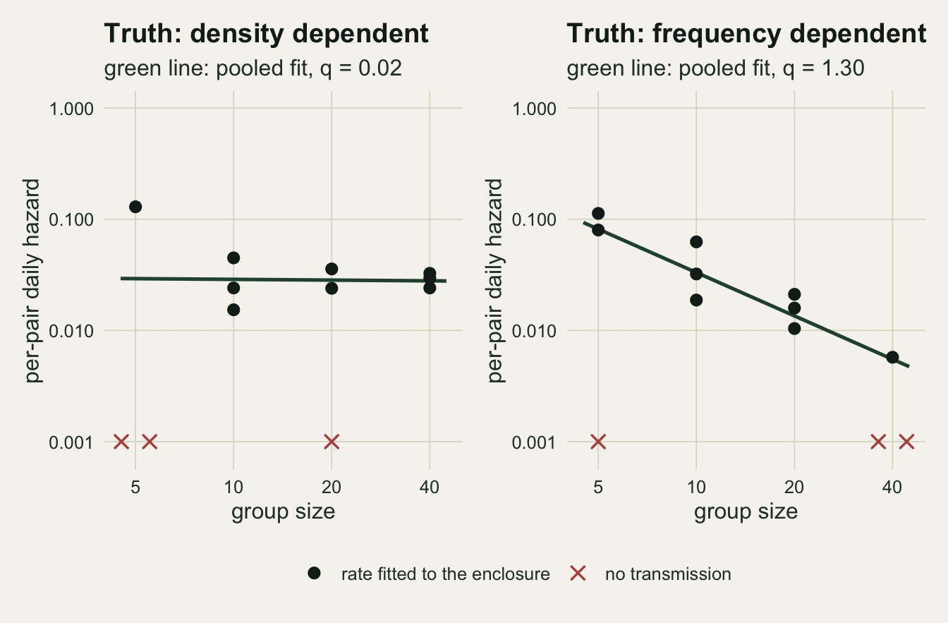
Eight enclosures: the range decides
Now the design question, with the budget held at eight enclosures. Four layouts: group sizes 8 and 12 with four enclosures each; sizes 5 and 20 with four each; sizes 5, 10, 20 and 40 with two each; and a fixed group of 20 in enclosures of area 1, 2, 4 and 8, two each, which contrasts density at fixed number instead of number at fixed area. A fifth layout gives the narrow pair of sizes twelve enclosures, to ask whether replication can stand in for range. Each runs under both forms and under the intermediate exponent of one half, with no enclosure variation. Two numbers per cell: how often the likelihood picks the true form, and how often the 95 per cent interval for the exponent contains both 0 and 1, so that the experiment cannot tell the forms apart.
n_exp_design <- 300   # experiments per cell, fixed before any rate was seen
designs <- list(
  list(label = "sizes 8, 12 (x4)", sizes = c(8, 12), reps = 4, area = 1, cov = "N"),
  list(label = "sizes 8, 12 (x6)", sizes = c(8, 12), reps = 6, area = 1, cov = "N"),
  list(label = "sizes 5, 20 (x4)", sizes = c(5, 20), reps = 4, area = 1, cov = "N"),
  list(label = "sizes 5 to 40 (x2)", sizes = c(5, 10, 20, 40), reps = 2, area = 1, cov = "N"),
  list(label = "20 animals, area 1 to 8 (x2)", sizes = 20, reps = 2, area = c(1, 2, 4, 8), cov = "A"))
q_set <- c(0, 0.5, 1)
set.seed(4304)
design_tab <- do.call(rbind, lapply(designs, function(ds) do.call(rbind, lapply(q_set, function(q) {
  dat <- sim_experiments(n_exp_design, ds$sizes, ds$reps, q, 0, ds$area)
  ff <- fit_day_level(dat, ds$cov)
  lo <- ff$q_hat - z95 * ff$se; hi <- ff$q_hat + z95 * ff$se
  data.frame(design = ds$label, q = q,
             pick_true = if (q == 0) mean(ff$pick_dd) else mean(!ff$pick_dd),
             pick_dd = mean(ff$pick_dd),
             both_in = mean(lo < 0 & hi > 1), excl_both = mean(lo > 0 & hi < 1),
             rej_true = mean(q < lo | q > hi), no_est = sum(!is.finite(ff$se)))
}))))
design_tab$design <- factor(design_tab$design, levels = rev(sapply(designs, `[[`, "label")))
dv <- function(lab, q, col) design_tab[design_tab$design == lab & design_tab$q == q, col]
lab_n4 <- designs[[1]]$label; lab_n6 <- designs[[2]]$label; lab_two <- designs[[3]]$label
lab_wide <- designs[[4]]$label; lab_area <- designs[[5]]$label
mcse_half <- sqrt(0.25 / n_exp_design)
rej_max <- max(design_tab$rej_true[design_tab$q != 0.5])
n_no_est <- sum(design_tab$no_est)
n_fitted <- n_exp_design * nrow(design_tab)
no_est_txt <- if (n_no_est == 0) sprintf("all %d fitted experiments returned a finite standard error", n_fitted) else
  sprintf("%d of the %d fitted experiments returned no finite standard error", n_no_est, n_fitted)
With sizes 8 and 12 the likelihood picks the true form in 0.74 of experiments under density dependence and 0.73 under frequency dependence, where a coin would score 0.5, and the interval holds both 0 and 1 in 0.75 and 0.75. A group of 12 is only one and a half times a group of 8, and on the log scale that contrast is short. Spending twelve enclosures on the same two sizes moves the pick rates to 0.79 and 0.80, and the interval still cannot separate the forms in 0.66 and 0.63.
Stretching the same eight enclosures over sizes 5 and 20 gives pick rates of 0.98 and 0.93; four sizes from 5 to 40 give 1.00 and 0.99, with the undecided interval down to 0.000 and 0.003. Varying area at a fixed group of 20 does as well as varying number: 0.990 and 0.993. What separates the forms is the ratio of densities, eight-fold in both of the wide layouts, not the number of enclosures. This equivalence is built into the simulator, which lets one exponent govern both number and area; an experiment that varies both can test that assumption, and one that varies only one of them cannot. The Monte Carlo standard error of a rate is at most 0.029 in these cells. With no enclosure variation, the Wald interval rejects the true exponent at most 0.063 of the time in any of the ten cells with q of 0 or 1; all 4500 fitted experiments returned a finite standard error.
dplot <- design_tab[design_tab$q != 0.5, ]
dplot$truth <- factor(ifelse(dplot$q == 0, "truth: density dependent", "truth: frequency dependent"))
p_pick <- ggplot(dplot, aes(pick_true, design, colour = truth, shape = truth)) +
  geom_vline(xintercept = 0.5, colour = te_body, linetype = "dashed", linewidth = 0.5) +
  geom_errorbar(aes(xmin = pick_true - 2 * sqrt(pick_true * (1 - pick_true) / n_exp_design),
                    xmax = pick_true + 2 * sqrt(pick_true * (1 - pick_true) / n_exp_design)),
                orientation = "y", width = 0.25, linewidth = 0.4, show.legend = FALSE) +
  geom_point(size = 2.6) +
  scale_colour_manual(values = c(te_forest, te_rust), name = NULL) +
  scale_shape_manual(values = c(16, 17), name = NULL) +
  coord_cartesian(xlim = c(0, 1.02)) +
  labs(x = "picks the true form", y = NULL, title = "Likelihood choice",
       subtitle = "dashed: a coin") +
  theme_datasheet() + theme(legend.position = "bottom")
p_both <- ggplot(dplot, aes(both_in, design, colour = truth, shape = truth)) +
  geom_point(size = 2.6) +
  scale_colour_manual(values = c(te_forest, te_rust), name = NULL) +
  scale_shape_manual(values = c(16, 17), name = NULL) +
  coord_cartesian(xlim = c(0, 1)) +
  labs(x = "intervals holding 0 and 1", y = NULL, title = "Undecided interval",
       subtitle = "the experiment cannot tell") +
  theme_datasheet() + theme(legend.position = "bottom", axis.text.y = element_blank())
(p_pick | p_both) + plot_layout(guides = "collect", widths = c(1.25, 1)) +
  plot_annotation(theme = theme_datasheet() + theme(legend.position = "bottom"))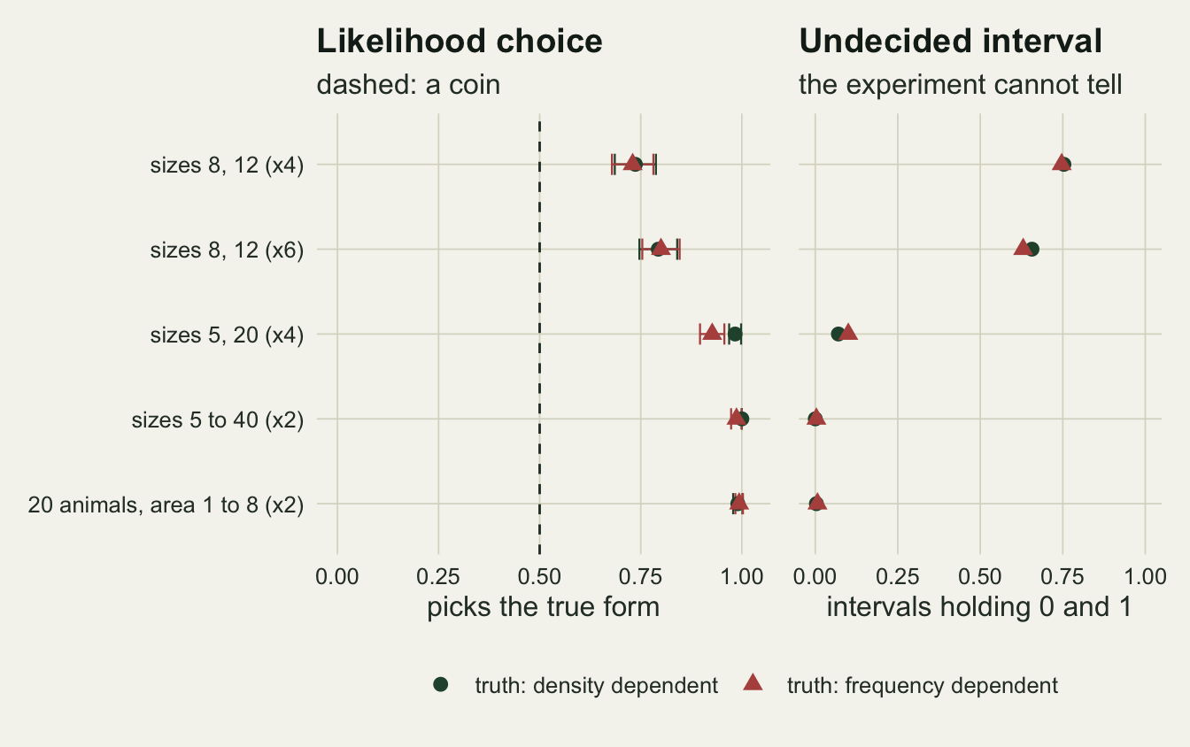
An intermediate exponent is not a vote
Smith and colleagues 2009 fitted transmission functions to field time series of cowpox in field voles and found the best-supported form between the two textbook ones. Under an exponent of one half the choice between density and frequency models has no right answer, and the design results say what the forced choice does with it.
With sizes 5 to 40 the likelihood calls the half-exponent density dependent in 0.55 of experiments, and with sizes 8 and 12 in 0.52: a split close to even in both, with the narrow design no more decisive than the wide one. The free exponent is where the designs differ. Its interval excludes both 0 and 1 in 0.56 of the wide experiments and 0.60 of the area experiments, against 0.000 with sizes 8 and 12. So an experiment that picks one of two fixed forms reports a winner whatever the truth; the free exponent with its interval is the result, and the two named forms are values it can be tested against.
Enclosures that differ break the day-level interval
Enclosures are not identical. Vegetation cover, burrow layout, the social rank of the index animal and the weather in one corner of the field all shift the rate at which an enclosure transmits. Give each enclosure its own transmission rate, lognormal with a standard deviation on the log scale from 0 to 0.6, and fit the same day-level GLM to the wide design with three and then six enclosures per size. A standard deviation of 0.6 means that an enclosure one standard deviation above the median transmits 1.8 times as fast as the median one.
n_exp_het <- 300
sd_grid <- c(0, 0.2, 0.4, 0.6)
het_cells <- expand.grid(sd_log = sd_grid, q = c(0, 1), reps = c(3, 6))
set.seed(4405)
kept <- list()
het_tab <- do.call(rbind, lapply(seq_len(nrow(het_cells)), function(i) {
  cc <- het_cells[i, ]
  dat <- sim_experiments(n_exp_het, c(5, 10, 20, 40), cc$reps, cc$q, cc$sd_log)
  ff <- fit_day_level(dat)
  if (cc$reps == 3 && cc$sd_log %in% c(0, 0.6))
    kept[[sprintf("q%g_sd%g", cc$q, cc$sd_log)]] <<- list(dat = dat, fit = ff, q = cc$q, sd_log = cc$sd_log)
  data.frame(cc, n_encl = 4 * cc$reps,
             rej_true = mean(abs(ff$q_hat - cc$q) > z95 * ff$se),
             pick_true = if (cc$q == 0) mean(ff$pick_dd) else mean(!ff$pick_dd),
             med_bias = median(ff$q_hat) - cc$q, sd_q = sd(ff$q_hat), med_se = median(ff$se),
             med_disp = median(ff$dispersion))
}))
hv <- function(q, s, r, col) het_tab[het_tab$q == q & het_tab$sd_log == s & het_tab$reps == r, col]
mcse_rej <- function(p) sqrt(p * (1 - p) / n_exp_het)
With no enclosure variation the Wald interval rejects the true exponent in 0.053 of density-dependent experiments and 0.063 of frequency-dependent ones, with twelve enclosures. A standard deviation of 0.2 already takes them to 0.11 and 0.10. At 0.6 the rates are 0.45 and 0.35, with Monte Carlo standard errors near 0.029. Meanwhile the likelihood still picks the true form in 0.90 and 0.90 of the same experiments. The point estimate survives; the interval around it is too narrow.
The reason is the one pseudoreplication and false positives in ecology measured for fish in tanks. Group size is a property of the enclosure, and so is the extra transmission rate. The day records inside an enclosure are sub-samples of one draw, but the binomial likelihood counts every day and every susceptible as independent information about the exponent. At a standard deviation of 0.6 the spread of the estimated exponent across experiments is 0.35 under density dependence, while the median model standard error is 0.14.
Doubling to 24 enclosures does not repair it. The rejection rates at a standard deviation of 0.6 become 0.47 and 0.36, because the model standard error shrinks with the extra days and animals at about the rate the real uncertainty shrinks with the extra enclosures. The usual overdispersion check does not see the problem either: the median Pearson dispersion of the day records is 1.14 under density dependence at 0.6, against 1.00 with no variation. A day with a handful of susceptibles has too little binomial variance to show a rate that is shared by all days of its enclosure.
There is also a small shift in the estimate. Its size is a median, and a median over 300 experiments is noisy, so the shift gets its own runs: 1000 fresh experiments per cell with twelve enclosures, keeping each enclosure’s log draw.
n_exp_big <- 1000   # experiments per cell, fixed before any rate was seen
set.seed(4407)
big <- list()
for (q in c(0, 1)) for (s_log in c(0, 0.6)) {
  dat <- sim_experiments(n_exp_big, c(5, 10, 20, 40), 3, q, s_log)
  big[[sprintf("q%g_sd%g", q, s_log)]] <- list(dat = dat, fit = fit_day_level(dat), q = q, sd_log = s_log)
}
mcse_median <- function(v) 1.2533 * sd(v) / sqrt(length(v))
shift_tab <- do.call(rbind, lapply(big[c("q0_sd0.6", "q1_sd0.6")], function(bc) {
  d <- bc$dat
  oracle <- irls_cloglog(d$new, d$S, log(d$N), log(d$I) + d$log_draw, d$exper)
  enc_key <- (d$exper - 1) * attr(d, "n_encl") + d$encl
  n_days <- tapply(d$new, enc_key, length)
  enc_N <- tapply(d$N, enc_key, function(v) v[1])
  enc_draw <- tapply(d$log_draw, enc_key, function(v) v[1])
  cors <- sapply(c(5, 10, 20, 40), function(n) cor(enc_draw[enc_N == n], n_days[enc_N == n]))
  data.frame(q = bc$q, naive = median(bc$fit$q_hat) - bc$q, naive_se = mcse_median(bc$fit$q_hat),
             oracle = median(-oracle$b) - bc$q, oracle_se = mcse_median(-oracle$b),
             cor5 = cors[1], cor10 = cors[2], cor20 = cors[3], cor40 = cors[4])
}))
sv <- function(q, col) shift_tab[shift_tab$q == q, col]
At a standard deviation of 0.6 the median exponent sits +0.074 from the truth under density dependence and -0.027 under frequency dependence, with Monte Carlo standard errors of 0.015 and 0.013. Enclosures whose draw was high burn through their susceptibles in a few days, so in large groups they contribute fewer day records than enclosures whose draw was low. Under density dependence the correlation between an enclosure’s log draw and its number of day records is -0.05 at a group of five, -0.48 at twenty and -0.62 at forty; under frequency dependence it is -0.24, -0.12 and -0.11. Under density dependence the day-level likelihood then sees a lower hazard in large groups than in small ones, which reads as a positive exponent; under frequency dependence the correlation is weaker in large groups and does not grow with group size, and the shift is small and of the other sign. Fitting with each enclosure’s true draw as an extra offset, which no real analysis can do, moves the median to -0.007 and -0.006 from the truth, with Monte Carlo standard errors of 0.006 and 0.007: the shift is gone in both cells.
het_tab$truth <- factor(ifelse(het_tab$q == 0, "truth: density dependent", "truth: frequency dependent"))
het_tab$encl_lab <- factor(sprintf("%d enclosures", het_tab$n_encl))
ggplot(het_tab, aes(sd_log, rej_true, colour = encl_lab, linetype = encl_lab)) +
  geom_hline(yintercept = 0.05, colour = te_body, linetype = "dashed", linewidth = 0.5) +
  geom_errorbar(aes(ymin = rej_true - 2 * mcse_rej(rej_true), ymax = rej_true + 2 * mcse_rej(rej_true)),
                width = 0.02, linewidth = 0.4, linetype = "solid", show.legend = FALSE) +
  geom_line(linewidth = 0.9) + geom_point(size = 2.2) +
  facet_wrap(~ truth) +
  scale_colour_manual(values = c(te_forest, te_gold), name = NULL) +
  scale_linetype_manual(values = c("solid", "longdash"), name = NULL) +
  scale_y_continuous(limits = c(0, NA)) +
  labs(x = "standard deviation of log transmission rate between enclosures",
       y = "share rejecting the true exponent",
       title = "The day records are not the replicates",
       subtitle = "dashed line: the nominal five per cent") +
  theme_datasheet() + theme(legend.position = "bottom",
                            strip.text = element_text(colour = te_ink, face = "bold"))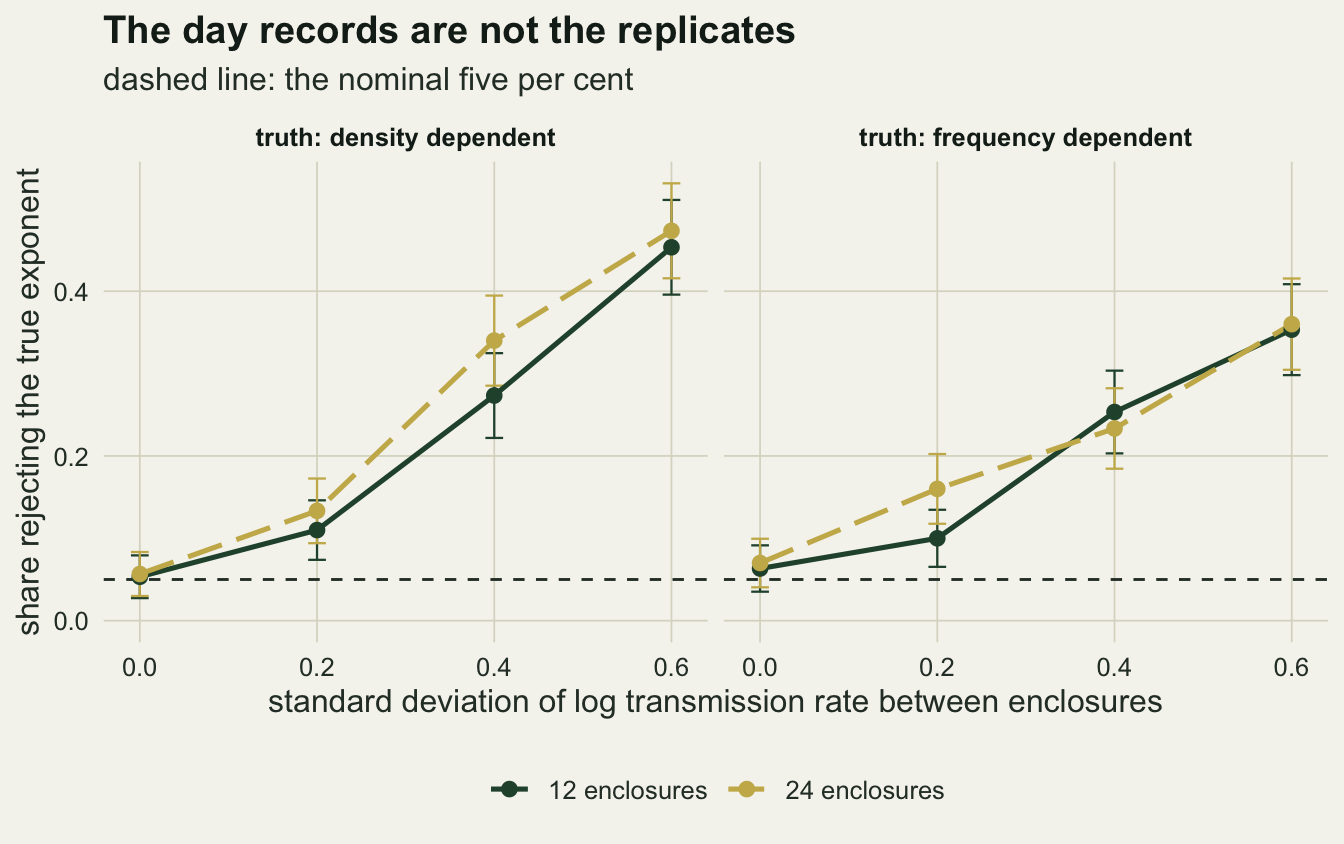
Repairs at the level of the enclosure
The enclosure is the replicate, so the uncertainty has to be measured across enclosures. Five intervals for the exponent, applied to twelve-enclosure experiments at standard deviations of 0 and 0.6. The day-level Wald interval is the reference. The quasi-binomial version inflates it by the Pearson dispersion when that exceeds one. The cluster sandwich sums the score over enclosures and uses a t quantile on 10 degrees of freedom, twelve enclosures minus two parameters. The delete-one-enclosure jackknife refits the model twelve times, each time without one enclosure, and uses the same t quantile. The cluster bootstrap resamples enclosures with replacement within each group size, as bootstrapping dependent data does with sites, refits, and takes the percentile interval.
n_boot <- 99; n_exp_fix <- 200   # fixed before any rate was seen
resample_q <- function(dat, fit, n_boot, chunk = 25) {
  n_encl <- attr(dat, "n_encl"); n_ex <- max(dat$exper)
  key <- (dat$exper - 1) * n_encl + dat$encl
  rows_by_key <- split(seq_len(nrow(dat)), factor(key, levels = seq_len(n_ex * n_encl)))
  strat <- tapply(dat$stratum, dat$encl, function(v) v[1])
  n_rep <- 1 + n_encl + n_boot
  out_jk <- matrix(NA, n_ex, n_encl); out_bs <- matrix(NA, n_ex, n_boot)
  for (start in seq(1, n_ex, by = chunk)) {
    ex_ids <- start:min(n_ex, start + chunk - 1)
    mult <- array(0, c(length(ex_ids), n_rep, n_encl))
    for (i in seq_along(ex_ids)) {
      m <- matrix(0, n_rep, n_encl); m[1, ] <- 1
      m[2:(n_encl + 1), ] <- 1 - diag(n_encl)
      if (n_boot > 0) for (k in unique(strat)) {
        ids <- which(strat == k)
        draws <- matrix(ids[sample.int(length(ids), n_boot * length(ids), TRUE)], n_boot)
        for (j in ids) m[(n_encl + 2):n_rep, j] <- rowSums(draws == j)
      }
      mult[i, , ] <- m
    }
    cmb <- expand.grid(i = seq_along(ex_ids), r = seq_len(n_rep), j = seq_len(n_encl))
    cmb$m <- mult[cbind(cmb$i, cmb$r, cmb$j)]
    cmb <- cmb[cmb$m > 0, ]
    idx <- rows_by_key[(ex_ids[cmb$i] - 1) * n_encl + cmb$j]; len <- lengths(idx)
    rows <- unlist(idx, use.names = FALSE)
    grp_raw <- rep((cmb$i - 1) * n_rep + cmb$r, len)
    ug <- sort(unique(grp_raw)); grp <- match(grp_raw, ug)
    gi <- (ug - 1) %/% n_rep + 1; gr <- (ug - 1) %% n_rep + 1
    fr <- irls_cloglog(dat$new[rows], dat$S[rows], log(dat$N[rows]), log(dat$I[rows]), grp,
                       mult = rep(cmb$m, len), a0 = fit$a_hat[ex_ids][gi],
                       b0 = fit$b_hat[ex_ids][gi])
    for (i in seq_along(ex_ids)) {
      sel <- gi == i
      out_jk[ex_ids[i], gr[sel][gr[sel] %in% 2:(n_encl + 1)] - 1] <- -fr$b[sel][gr[sel] %in% 2:(n_encl + 1)]
      if (n_boot > 0) out_bs[ex_ids[i], ] <- -fr$b[sel][gr[sel] > n_encl + 1]
    }
  }
  list(jk = out_jk, bs = out_bs)
}
method_lev <- c("day-level Wald", "day-level quasi", "cluster sandwich, t",
                "enclosure jackknife, t", "cluster bootstrap")
set.seed(4506)
boot_tab <- do.call(rbind, lapply(kept, function(kc) {
  keep_ex <- kc$dat$exper <= n_exp_fix
  dat <- kc$dat[keep_ex, ]; attr(dat, "n_encl") <- attr(kc$dat, "n_encl")
  f <- kc$fit[seq_len(n_exp_fix), ]
  rs <- resample_q(dat, f, n_boot)
  G <- attr(dat, "n_encl"); q <- kc$q
  se_jk <- sqrt((G - 1) / G * rowSums((rs$jk - rowMeans(rs$jk))^2))
  bs_lo <- apply(rs$bs, 1, quantile, 0.025); bs_hi <- apply(rs$bs, 1, quantile, 0.975)
  data.frame(q = q, sd_log = kc$sd_log, method = method_lev[5], rej = mean(q < bs_lo | q > bs_hi),
             rej_other = NA, rej_half = NA, n = n_exp_fix, jk_ratio = NA, jk_spread = NA,
             bs_ratio = median(apply(rs$bs, 1, sd) / se_jk))
}))
enc_tab <- do.call(rbind, lapply(big, function(bc) {
  dat <- bc$dat; f <- bc$fit
  rs <- resample_q(dat, f, 0)
  G <- attr(dat, "n_encl"); q <- bc$q
  crit_t <- qt(0.975, G - 2)
  se_jk <- sqrt((G - 1) / G * rowSums((rs$jk - rowMeans(rs$jk))^2))
  half <- list(z95 * f$se,
               qt(0.975, f$n_row - 2) * f$se * sqrt(pmax(1, f$dispersion)),
               crit_t * f$se_cr, crit_t * se_jk)
  miss <- function(target) sapply(half, function(h) mean(abs(f$q_hat - target) > h))
  data.frame(q = q, sd_log = bc$sd_log, method = method_lev[1:4], rej = miss(q),
             rej_other = miss(1 - q), rej_half = miss(0.5), n = n_exp_big,
             jk_ratio = median(se_jk / f$se_cr), jk_spread = median(se_jk) / sd(f$q_hat),
             bs_ratio = NA)
}))
repair_tab <- rbind(enc_tab, boot_tab)
repair_tab$method <- factor(repair_tab$method, levels = method_lev)
rv <- function(q, s, k, col = "rej") repair_tab[repair_tab$q == q & repair_tab$sd_log == s &
                                                repair_tab$method == method_lev[k], col]
mcse_big <- sqrt(0.05 * 0.95 / n_exp_big); mcse_fix <- sqrt(0.05 * 0.95 / n_exp_fix)
bs_ratio_med <- median(boot_tab$bs_ratio)
jk_ratio_med <- median(enc_tab$jk_ratio)
jk_spread_rng <- range(enc_tab$jk_spread)
bs_range <- range(boot_tab$rej)
sand_range <- range(enc_tab$rej[enc_tab$method == method_lev[3] & enc_tab$sd_log == 0])
sand_z <- (sand_range[2] - 0.05) / mcse_big
jk_dev <- max(abs(enc_tab$rej[enc_tab$method == method_lev[4]] - 0.05)) / mcse_big
The first four intervals are computed on the 1000 experiments per cell from the shift runs above, where the Monte Carlo standard error of a rate near five per cent is 0.0069. The bootstrap refits every experiment once per resample, so it runs on the first 200 experiments of the matching heterogeneity cells, with a Monte Carlo standard error of 0.015 near five per cent. At a standard deviation of 0.6, the quasi-binomial interval rejects the true exponent in 0.37 of density-dependent and 0.31 of frequency-dependent experiments, hardly better than the plain Wald interval, which rejects in 0.43 and 0.34 on these runs (0.45 and 0.35 on the 300 experiments per cell above), as the dispersion figures above predicted. The cluster sandwich brings the rates to 0.101 and 0.104, still above nominal. Without enclosure variation it rejects in 0.058 and 0.083; the higher of the two is 4.8 Monte Carlo standard errors above five per cent. Twelve clusters are few for a sandwich estimator, which is the problem Cameron, Gelbach and Miller 2008 describe.
The jackknife is the repair that comes closest. Its rejection rates are 0.038 and 0.046 without enclosure variation and 0.052 and 0.045 at 0.6 (density then frequency dependence); the largest of the four departures from five per cent is 1.7 Monte Carlo standard errors. Its median standard error is 0.98 to 1.01 times the spread of the estimate across experiments, so it measures the real uncertainty rather than padding it, and it is a median 1.23 times the sandwich value.
An interval that holds its level can still be too wide to decide anything. At a standard deviation of 0.6 the jackknife interval excludes the wrong textbook form (an exponent of 1 when the truth is 0, and 0 when it is 1) in 0.60 of density-dependent and 0.68 of frequency-dependent experiments, against 0.80 and 0.85 for the sandwich, whose extra reach is bought with its excess false rejections. It excludes an exponent of one half in 0.18 and 0.28. Without enclosure variation the jackknife excludes the wrong form in 0.999 and 0.963, and one half in 0.83 and 0.72, against 0.95 and 0.89 for the Wald interval, which is valid there. The loss is the honest price of twelve replicates.
A binomial or quasi-binomial model on enclosure totals is not among the repairs: collapsing the days throws away the depletion of susceptibles that the chain binomial uses to separate the forms, and it was not measured here.
The cluster bootstrap fails at this size. It rejects the true exponent in 0.165 to 0.215 of experiments, and it does so even without enclosure variation. Resampling three enclosures with replacement from three estimates the variance of a mean of three with divisor three instead of two, which alone would shrink the spread to 0.82 of its proper size; here the bootstrap standard deviation is a median 0.77 of the jackknife standard error. The cluster bootstrap in that post resampled twenty sites; three enclosures per group size is a different regime.
repair_tab$truth <- factor(ifelse(repair_tab$q == 0, "density dependent", "frequency dependent"))
repair_tab$spread <- factor(sprintf("between-enclosure sd %.1f", repair_tab$sd_log))
repair_tab$method <- factor(repair_tab$method, levels = rev(method_lev))
ggplot(repair_tab, aes(rej, method, colour = truth, shape = truth)) +
  geom_vline(xintercept = 0.05, colour = te_body, linetype = "dashed", linewidth = 0.5) +
  geom_errorbar(aes(xmin = rej - 2 * sqrt(rej * (1 - rej) / n),
                    xmax = rej + 2 * sqrt(rej * (1 - rej) / n)),
                orientation = "y", width = 0.25, linewidth = 0.4,
                position = position_dodge(width = 0.5), show.legend = FALSE) +
  geom_point(size = 2.6, position = position_dodge(width = 0.5)) +
  facet_wrap(~ spread) +
  scale_colour_manual(values = c(te_forest, te_rust), name = "truth") +
  scale_shape_manual(values = c(16, 17), name = "truth") +
  coord_cartesian(xlim = c(0, NA)) +
  labs(x = "share rejecting the true exponent", y = NULL,
       title = "Twelve enclosures, five intervals",
       subtitle = "dashed line: the nominal five per cent") +
  theme_datasheet() + theme(legend.position = "bottom",
                            strip.text = element_text(colour = te_ink, face = "bold"))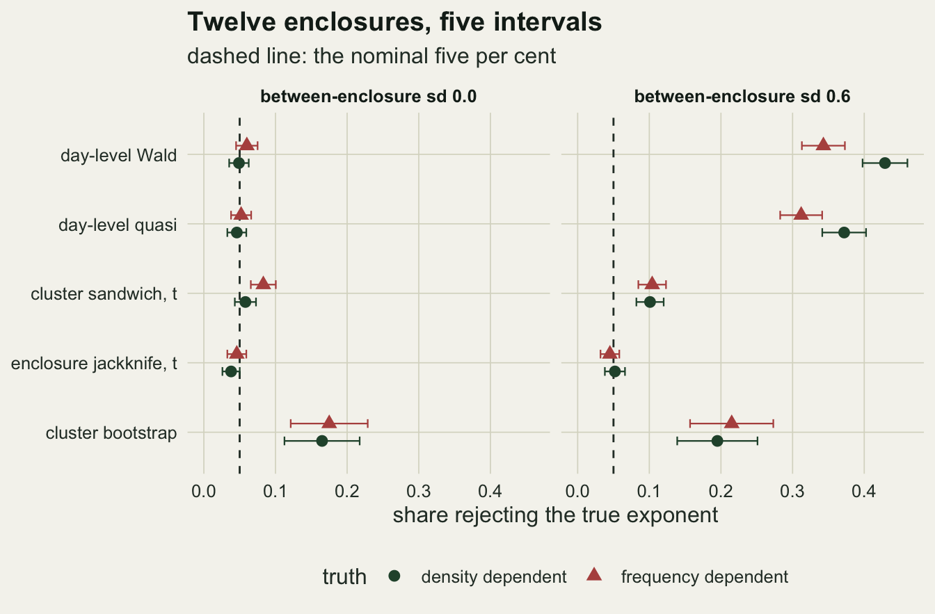
What to report
Report the exponent with its interval, not the name of the winning form. The likelihood comparison of two fixed forms always returns a winner, and under an intermediate exponent it returns either one at a rate close to a coin.
Give the range of group sizes, or of areas, as the ratio of the largest density to the smallest. That ratio decides whether the experiment could have told the forms apart, and a reader cannot recover it from the number of enclosures.
Give the number of enclosures as the sample size and compute the interval across enclosures. With twelve enclosures the delete-one-enclosure jackknife on a t quantile was the only interval here within two Monte Carlo standard errors of its nominal level both with and without enclosure variation; the day-level interval, with or without a dispersion correction, was not, and neither was a stratified cluster bootstrap with three enclosures per size. A random effect of enclosure in a binomial GLMM is the model-based route to the same end, with its own small-sample questions at twelve levels. With the interval computed across enclosures and a between-enclosure standard deviation of 0.6, twelve enclosures over sizes 5 to 40 rejected the wrong form in only 0.60 and 0.68 of experiments: the eight-fold range is necessary, not sufficient.
Say how infection was observed. Daily status of every animal is what makes the day-level likelihood possible, and it is rarely what a field experiment gets.
Honest limits
The simulated animals mix homogeneously within an enclosure and the exponent is the same power law at every group size. Real contact structure changes with group size in ways a single exponent does not capture, including territoriality that sets in above some density. Smith and colleagues 2009 found intermediate forms in field data, and Begon and colleagues 2002 note that the two forms are statements about how contacts scale with density and number, which an enclosure experiment manipulates only over the range it covers.
Infection status is known every day, with no latent period and no test error. Field experiments usually see seroconversion at trapping intervals, which turns the daily chain binomial into interval-censored data and loses information, so every rate above is a best case.
Between-enclosure variation is a lognormal draw that is independent of group size. If larger groups also differ in something that changes transmission, such as the proportion of cover per animal, the variation is confounded with the contrast and no interval repairs that.
The bootstrap was measured on 200 experiments per cell with 99 resamples, a small number for percentile limits; its failure is large enough that neither choice explains it. The other intervals and the shift used 1000 experiments per cell. Only a lognormal spread of 0 or 0.6 was tried for the repairs, only the wide twelve-enclosure layout, and the power of the jackknife was not measured for 24 enclosures.
The area design holds 20 animals at four areas. It matched the number design here, but it has its own practical problems, since enclosure area changes cover, food per animal and the chance that animals meet at all, and none of that is simulated.
References
McCallum H, Barlow N, Hone J 2001 Trends in Ecology and Evolution 16(6):295-300 (10.1016/S0169-5347(01)02144-9)
Begon M, Bennett M, Bowers RG, French NP, Hazel SM, Turner J 2002 Epidemiology and Infection 129(1):147-153 (10.1017/S0950268802007148)
Smith MJ, Telfer S, Kallio ER, Burthe S, Cook AR, Lambin X, Begon M 2009 Proceedings of the National Academy of Sciences 106(19):7905-7909 (10.1073/pnas.0809145106)
Cameron AC, Gelbach JB, Miller DL 2008 Review of Economics and Statistics 90(3):414-427 (10.1162/rest.90.3.414)