---
title: "Checking an epidemic model"
description: "Three checks for disease models in R: density versus frequency-dependent transmission, estimating R0 from the growth rate, and why superspreading breaks mixing."
date: "2026-07-05 13:00"
categories: [ecology tutorial, R, disease ecology, model diagnostics, theoretical ecology]
image: thumbnail.png
image-alt: "The reproduction number depending on host density under one transmission assumption but flat under another, the choice that decides whether culling works."
---
```{r setup}
#| code-fold: true
#| code-summary: "Setup: packages, colours and plot theme"
#| results: hide
#| message: false
#| warning: false
knitr::opts_chunk$set(echo = TRUE, message = FALSE, warning = FALSE,
                      dev = "png", dpi = 120, fig.path = "figures/",
                      fig.width = 7, fig.height = 4.4)
library(ggplot2)
theme_te <- theme_minimal(base_size = 12) +
  theme(panel.background = element_rect(fill = "#f5f4ee", colour = NA),
        plot.background  = element_rect(fill = "#f5f4ee", colour = NA),
        panel.grid.minor = element_blank(),
        plot.title = element_text(face = "bold", size = 12))
theme_set(theme_te)
col_a <- "#3a6b52"; col_b <- "#b5651d"; col_ref <- "#555555"

b <- 0.002; gamma <- 0.1; beta_fd <- 0.4
r_obs <- 0.297
R0_from_r <- function(D) 1 + r_obs*D
set.seed(170)
kh <- rpois(5000, 5)
ko <- rnbinom(5000, mu = 5, size = 0.3)
eff <- function(k) mean(k^2)/mean(k)
ratio_h <- eff(kh)/mean(kh); ratio_o <- eff(ko)/mean(ko)
top20 <- function(k) sum(sort(k, decreasing = TRUE)[1:1000])/sum(k)
```
A disease model is a set of assumptions wearing the clothes of a mechanism, and the assumptions are load-bearing. Two epidemic models can fit the same outbreak curve and disagree completely about whether culling the host will help, what the reproduction number is, and how likely the next introduction is to take off. These three checks are the ones that most often separate a disease model that informs management from one that misleads it.
## Check 1: how does transmission scale?
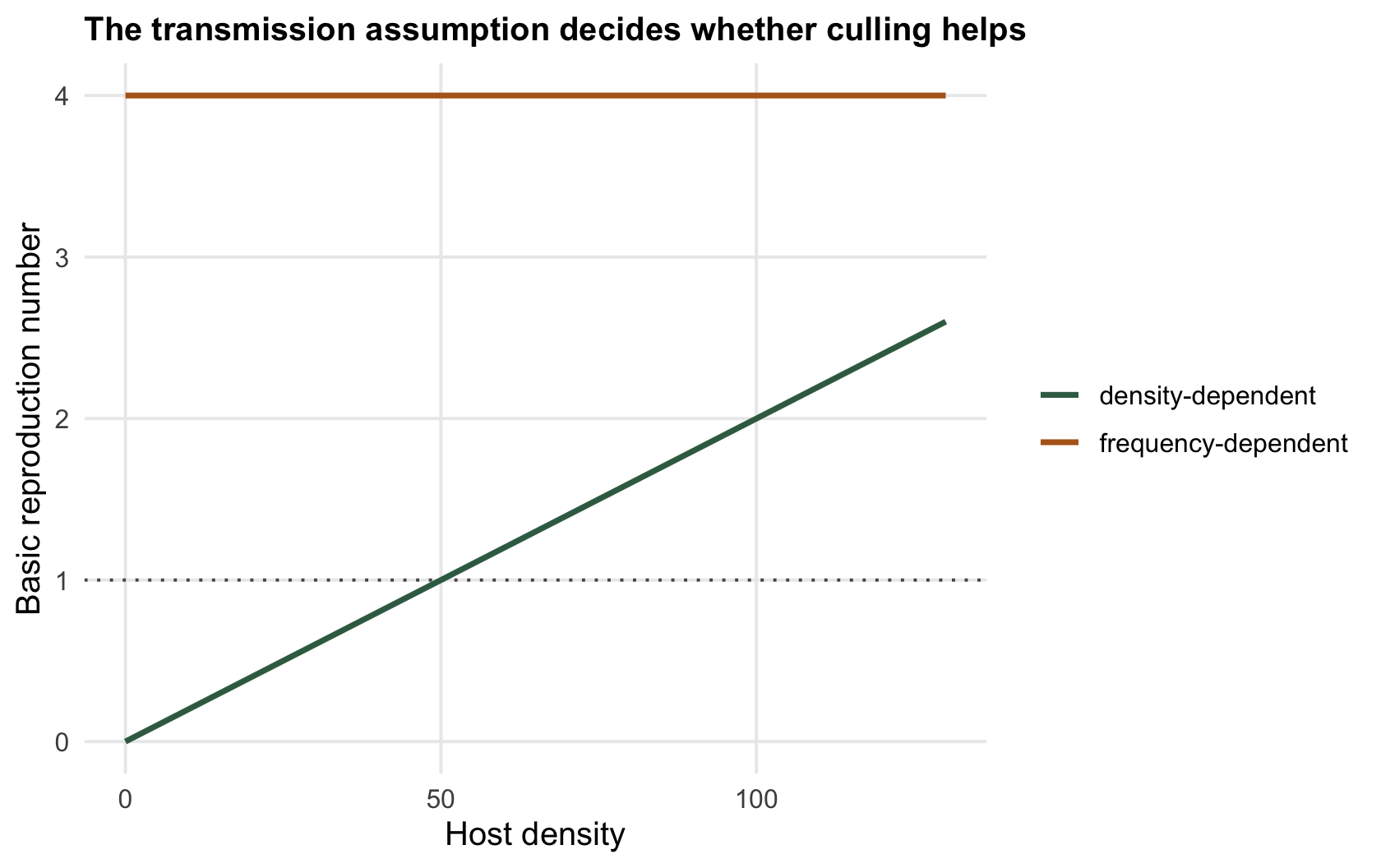
This is the choice that governs everything downstream. If transmission is density-dependent, the contact rate rises with how crowded the hosts are, and there is a threshold host density below which the pathogen cannot invade, so thinning the population works. If transmission is frequency-dependent, each host has roughly a fixed number of contacts regardless of density, the reproduction number does not depend on host numbers, and thinning the population does nothing. Same infection, same data, opposite management.
```{r transmission}
b <- 0.002; gamma <- 0.1; beta_fd <- 0.4
R0_density   <- function(N) b*N/gamma        # density-dependent: rises with N
R0_frequency <- function(N) beta_fd/gamma    # frequency-dependent: flat in N
rbind(density_dependent   = sapply(c(30, 60, 120), R0_density),
      frequency_dependent = sapply(c(30, 60, 120), R0_frequency))
```
Under density dependence the reproduction number climbs from below one to well above it as host density quadruples; under frequency dependence it stays flat at four whatever the density. A study that assumes the wrong one will either promise that a cull clears the disease when it cannot, or dismiss density control that would actually work. The transmission form is almost never identifiable from a single epidemic curve, so it has to be argued from the biology of how the pathogen spreads, not read off the fit.
```{r fig-transmission}
#| fig-cap: "The reproduction number against host density under the two transmission assumptions. Density-dependent (green) crosses the threshold and keeps rising, so culling can push it below one; frequency-dependent (ochre) is flat, so culling never does."
#| fig-alt: "A rising green line and a flat ochre line of reproduction number against host density, with a dotted line at one; only the green line crosses it."
Ng <- seq(0, 130, 1)
dt <- rbind(data.frame(N = Ng, R0 = R0_density(Ng), type = "density-dependent"),
            data.frame(N = Ng, R0 = R0_frequency(Ng), type = "frequency-dependent"))
ggplot(dt, aes(N, R0, colour = type)) +
  geom_hline(yintercept = 1, colour = col_ref, linetype = "dotted") +
  geom_line(linewidth = 1) +
  scale_colour_manual(values = c("density-dependent" = col_a, "frequency-dependent" = col_b)) +
  labs(x = "Host density", y = "Basic reproduction number", colour = NULL,
       title = "The transmission assumption decides whether culling helps")
```
## Check 2: what infectious period went into R0?
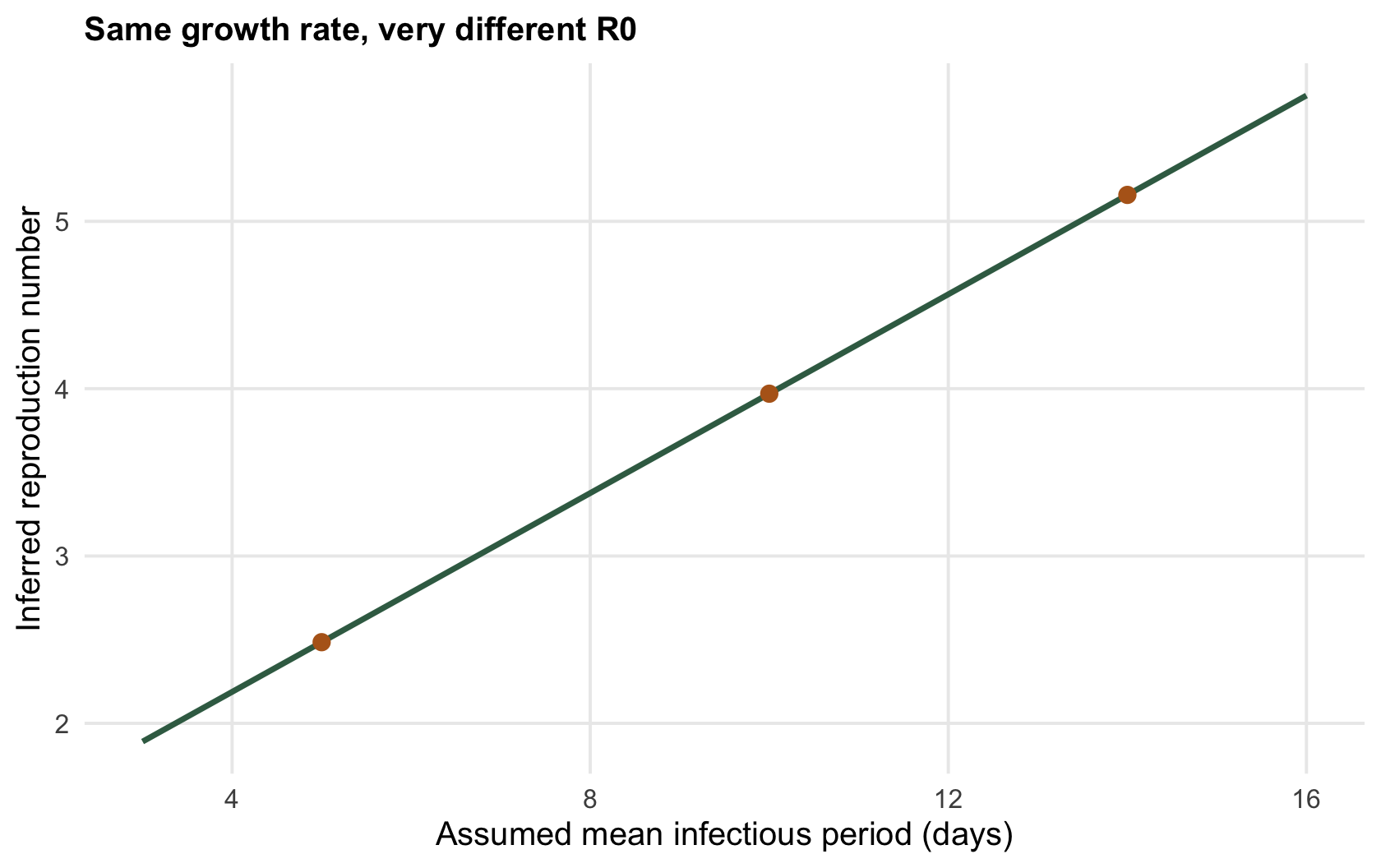
The reproduction number is often estimated from how fast cases grow early in an outbreak, through the relationship that ties it to the exponential growth rate and the infectious period. That relationship is only as good as the infectious period you assume, and getting the period wrong drags the reproduction number with it. Take one observed growth rate and turn the assumed infectious period.
```{r growth}
r_obs <- 0.297                          # observed early exponential growth rate
R0_from_r <- function(D) 1 + r_obs*D    # D = assumed mean infectious period (days)
c(period_5 = R0_from_r(5), period_10 = R0_from_r(10), period_14 = R0_from_r(14))
```
The very same growth rate gives a reproduction number of `r sprintf("%.1f", R0_from_r(5))` if the infectious period is five days, `r sprintf("%.1f", R0_from_r(10))` at ten days, and `r sprintf("%.1f", R0_from_r(14))` at fourteen. That is the difference between a herd immunity target of sixty per cent and one over eighty per cent, from a number that is usually assumed rather than measured. A reproduction number quoted without the generation interval that produced it is only half a result.
```{r fig-growth}
#| fig-cap: "The reproduction number inferred from one fixed growth rate, against the assumed infectious period. The same outbreak data yield very different reproduction numbers depending on a period that is often guessed."
#| fig-alt: "A rising line of inferred reproduction number against assumed infectious period, spanning from just under two to nearly six."
Dg <- seq(3, 16, 0.5)
dg <- data.frame(D = Dg, R0 = R0_from_r(Dg))
ggplot(dg, aes(D, R0)) +
  geom_line(colour = col_a, linewidth = 1) +
  geom_point(data = data.frame(D = c(5, 10, 14), R0 = R0_from_r(c(5, 10, 14))),
             aes(D, R0), colour = col_b, size = 2.4) +
  labs(x = "Assumed mean infectious period (days)", y = "Inferred reproduction number",
       title = "Same growth rate, very different R0")
```
## Check 3: does everyone really mix the same?
The basic model assumes homogeneous mixing: every host has the same contact rate, so the reproduction number is the average number of secondary cases. Real contact networks are nothing like that; a few hosts have far more contacts than the rest, and those superspreaders dominate transmission. When contacts are that uneven, the reproduction number is not set by the mean number of contacts but by a quantity that also carries their variance, so the naive estimate from the average badly understates the truth.
```{r heterogeneity}
set.seed(170)
kh <- rpois(5000, 5)                    # homogeneous: everyone near the mean
ko <- rnbinom(5000, mu = 5, size = 0.3) # superspreading: same mean, heavy tail
eff <- function(k) mean(k^2)/mean(k)    # the contact number that actually drives R0
c(mean_contacts = mean(ko),
  effective_homogeneous = eff(kh),
  effective_superspreading = eff(ko))
```
Both populations average five contacts, but the effective contact number that drives transmission is `r sprintf("%.1f", eff(kh))` under homogeneous mixing and `r sprintf("%.1f", eff(ko))` under superspreading: the reproduction number computed from the mean underestimates the real one by more than fourfold when the tail is heavy. The signature is concentration, the busiest fifth of hosts account for `r sprintf("%.0f", 100*top20(ko))` per cent of all contacts under superspreading against `r sprintf("%.0f", 100*top20(kh))` per cent when mixing is even. Heterogeneity cuts both ways for management: it raises the reproduction number, but it also means that targeting the few high-contact hosts pays off far more than treating everyone equally, an option the homogeneous model cannot even represent.
## The weight of the assumptions
Three checks, one lesson: an epidemic model's answer is mostly its assumptions, and the assumptions are choices, not measurements. Density or frequency transmission decides whether culling works; the assumed infectious period sets the reproduction number and the immunity target; homogeneous mixing hides both the true reproduction number and the payoff from targeting superspreaders. None of this makes the [SIR framework](../the-sir-epidemic-model/) wrong; it makes it a scaffold whose predictions are only as trustworthy as the biology poured into it. The discipline is to state each assumption, ask what would change if it were the other way, and reach for data or the natural history of the host and pathogen before quoting a number as if the model had measured it.
## References
- McCallum H, Barlow N, Hone J 2001. Trends in Ecology and Evolution 16(6):295-300 (10.1016/S0169-5347(01)02144-9).
- Lloyd-Smith JO, Schreiber SJ, Kopp PE, Getz WM 2005. Nature 438(7066):355-359 (10.1038/nature04153).
- Wallinga J, Lipsitch M 2007. Proceedings of the Royal Society B 274(1609):599-604 (10.1098/rspb.2006.3754).
## Related tutorials
- [The SIR epidemic model](../the-sir-epidemic-model/)
- [R0 and herd immunity](../r0-and-herd-immunity/)
- [Host density and endemic disease](../host-density-and-endemic-disease/)
- [Density or frequency transmission in enclosures](../density-or-frequency-dependent-transmission/)