library(ggplot2)
library(patchwork)

te_paper  <- "#f5f4ee"
te_ink    <- "#16241d"
te_body   <- "#2c3a31"
te_forest <- "#275139"
te_rust   <- "#b5534e"
te_gold   <- "#c9b458"
te_line   <- "#dad9ca"

theme_datasheet <- function() {
  theme_minimal(base_size = 12) +
    theme(plot.background  = element_rect(fill = te_paper, colour = NA),
          panel.background = element_rect(fill = te_paper, colour = NA),
          panel.grid.major = element_line(colour = te_line, linewidth = 0.3),
          panel.grid.minor = element_blank(),
          text             = element_text(colour = te_body),
          plot.title       = element_text(colour = te_ink, face = "bold"),
          plot.subtitle    = element_text(colour = te_body),
          axis.text        = element_text(colour = te_body))
}Fertility control versus culling in R
R
population dynamics
wildlife management
density dependence
simulation
ecology tutorial
Culling and permanent sterilisation at the same treatment rate share one long-run population. Measuring in R the years and animals handled that separate them.
A park authority has too many deer in a small suburban reserve and two proposals on the table. One is a marksman team that removes a fixed share of the females every winter. The other is a darting team that treats the same share with a permanent contraceptive and leaves every animal in place. The public meeting treats this as a question about ethics and cost. Underneath both sits a question about population dynamics that can be answered exactly: if the same fraction of females is treated each year, where does the population end up, and how long does it take to get there?
The population-control posts linked here all remove animals. The post on host density and endemic disease ends on culling a host population below a transmission threshold and warns that the threshold is a modelling choice; the post on checking an epidemic model shows that the way transmission scales decides whether culling works at all; and the post on stochastic dynamic programming for harvest derives an optimal removal rule for a fished stock. None of them has a lever that leaves the animal alive and takes away only its offspring. That lever changes one thing the removal models never have to think about: sterile animals go on eating, and if they count in the density feedback they go on suppressing the recruitment of the fertile ones.
The density feedback here is the plain compensation that the post on detecting density dependence tests for in a count series, and the bookkeeping is the one the post on Leslie matrix population models uses: a stated census point, and survival and recruitment applied in a fixed order. With both in place, a short calculation shows that the two proposals arrive at the same long-run population. The headline is not new. Barlow, Kean and Briggs (1997) found with logistic models that culling in general reduces density faster than sterilisation while the long-run suppression at the same level of control is similar, and that the mating system changes how well sterilisation works; Hobbs, Bowden and Baker (2000) built stage-structured models of fertility control for ungulates. This post reproduces that result in a model small enough to derive by hand and quantifies it: an exact derivation of the shared census, how the lag depends on survival and on the census point, the animals handled on the way, the loss of the breeding core under demographic noise, and which assumption turns a slower answer into a different one.
One female population, two levers, one census
The model follows females only. At the census each year there are fertile and sterile adults. Treatment happens straight after the census, recruitment happens in the breeding season with a Beverton-Holt density effect on every animal present, adults survive the year, and recruits join the fertile class before the next census. Culling removes a fraction h of the untreated females. Sterilisation marks the same fraction of the untreated females as permanently sterile. In both cases the census population is counted immediately after the treatment, so it is the number of animals actually living in the reserve through the year, and the same count is used for both levers. That choice is not neutral for the timing, and a later section shows what moves when the count is taken before treatment.
Two design constants are fixed across every life history. The maximum annual multiplier of an uncrowded, untreated population, adult survival plus recruits per female, is 1.5, so a species with low adult survival compensates with higher recruitment. The untreated equilibrium is 1000 females, which sets the strength of the density effect for each survival value. Both were chosen before any run, so that the life histories differ in adult survival and in the recruitment that compensates for it, with the same uncrowded multiplier and the same untreated size. The density coefficient, and so the equilibrium under treatment, changes with them.
lam_max  <- 1.5     # adult survival + recruits per female, uncrowded
k_cap    <- 1000    # untreated equilibrium, females
h_crit   <- 1 - 1 / lam_max
half_pop <- k_cap / 2
s_show   <- c(0.60, 0.75, 0.85, 0.95)

demog <- function(s_a) {
  r0 <- lam_max - s_a
  list(r0 = r0, cc = (r0 / (1 - s_a) - 1) / k_cap)
}

# lever: "cull", "sterile" (permanent) or "season" (one breeding season)
project <- function(s_a, h, n_year, lever = "cull", sterile_in_dd = TRUE,
                    bonus = 0, demographic = FALSE) {
  n_cell <- max(length(s_a), length(h))
  s_a <- rep_len(s_a, n_cell); h <- rep_len(h, n_cell)
  dm    <- demog(s_a)
  s_st  <- s_a + bonus
  pre_f <- rep(k_cap, n_cell); ster <- rep(0, n_cell); done <- rep(0, n_cell)
  pop <- fert <- hand <- matrix(NA_real_, n_cell, n_year)
  for (yr in seq_len(n_year)) {
    treated  <- if (demographic) rbinom(n_cell, pre_f, h) else h * pre_f
    done     <- done + treated
    fert_now <- pre_f - treated
    ster <- switch(lever, cull = 0, season = treated, sterile = ster + treated)
    pop[, yr] <- fert_now + ster; fert[, yr] <- fert_now; hand[, yr] <- done
    dens   <- fert_now + if (sterile_in_dd) ster else 0
    mu_rec <- dm$r0 * fert_now / (1 + dm$cc * dens)
    if (demographic) {
      live_f   <- rbinom(n_cell, fert_now, s_a)
      live_s   <- rbinom(n_cell, ster, s_st)
      recruits <- rpois(n_cell, mu_rec)
    } else {
      live_f <- s_a * fert_now; live_s <- s_st * ster; recruits <- mu_rec
    }
    if (lever == "season") {
      pre_f <- live_f + live_s + recruits; ster <- 0
    } else {
      pre_f <- live_f + recruits; ster <- live_s
    }
  }
  list(pop = pop, fert = fert, hand = hand)
}

first_below <- function(pop_mat, level = half_pop) {
  apply(pop_mat, 1, function(v) {
    w <- which(v <= level)
    if (length(w)) w[1] else NA_integer_
  })
}
The effort currency is the same for both levers: animals handled is the number of untreated females taken or treated in a year, which is h times the untreated females present at the treatment. A female already carrying a permanent sterilant is not handled again. A culled female is gone, so every female present is untreated.
The same end point, derived
Write P for the census population, s for adult survival, r0 for recruits per female when uncrowded and c for the density coefficient. Under culling every animal at the census is fertile, and one year later the census is the survivors and recruits, less the next cull:
P(t+1) = (1 - h) (s + r0 / (1 + c P(t))) P(t)
Under sterilisation the fertile females F follow the same kind of recursion, because only they breed and only the untreated survivors and recruits can be treated next year, while the recruitment term still sees the whole census population:
F(t+1) = (1 - h) (s + r0 / (1 + c P(t))) F(t)
The multiplier in brackets is identical. A positive equilibrium requires it to equal one, which happens at one value of P only, and that value is the same for both levers:
P* = (r0 / (1 / (1 - h) - s) - 1) / c
It exists when h is below the critical rate 1 - 1 / (s + r0), which with the multiplier fixed at 1.5 is 0.333 for every life history here. The sterile animals are part of P*: at the sterilisation equilibrium the census holds the same total, but fewer of them breed.
p_star <- function(s_a, h) {
  dm <- demog(s_a)
  pmax((dm$r0 / (1 / (1 - h) - s_a) - 1) / dm$cc, 0)
}
f_star <- function(s_a, h, s_st = s_a) p_star(s_a, h) / (1 + h / ((1 - h) * (1 - s_st)))

grid_id  <- expand.grid(s_a = seq(0.50, 0.95, by = 0.05), h = seq(0.05, 0.30, by = 0.05))
n_long   <- 3000
long_cul <- project(grid_id$s_a, grid_id$h, n_long, "cull")$pop[, n_long]
long_ste <- project(grid_id$s_a, grid_id$h, n_long, "sterile")$pop[, n_long]
closed   <- p_star(grid_id$s_a, grid_id$h)
gap_cul  <- max(abs(long_cul - closed))
gap_ste  <- max(abs(long_ste - closed))
n_id     <- nrow(grid_id)

fert_share <- f_star(s_show, 0.2) / p_star(s_show, 0.2)
Running both recursions for 3000 years on a grid of 60 combinations of adult survival and treatment rate, the largest distance between the simulated census and the closed form is 6.82e-13 animals for culling and 1.02e-12 for sterilisation, which is rounding error. At a treatment rate of 0.2, the fertile share of the sterilisation equilibrium is 0.62 at adult survival 0.60 and 0.17 at 0.95. Long-lived sterile animals pile up, and they do the suppressing that culled animals would have done by being absent.
The price is time, and it grows with survival
n_show <- 40
traj_c <- project(s_show, 0.2, n_show, "cull")
traj_s <- project(s_show, 0.2, n_show, "sterile")
t50_c  <- first_below(traj_c$pop)
t50_s  <- first_below(traj_s$pop)
y10_c3 <- project(s_show, 0.3, 10, "cull")$pop[, 10]
y10_s3 <- project(s_show, 0.3, 10, "sterile")$pop[, 10]
eq_02  <- p_star(s_show, 0.2)
min_s85 <- min(traj_s$pop[3, ])
yr_min_s85 <- which.min(traj_s$pop[3, ])
At a treatment rate of 0.2 the culled population falls below half of its starting size in 5, 5, 4 and 4 years for adult survival 0.60, 0.75, 0.85 and 0.95. The sterilised population takes 8, 9, 11 and 20 years. Culling gets faster as survival rises, because the fixed untreated equilibrium means a long-lived species has weaker recruitment to refill the gap. Sterilisation gets slower, because the treated animals do not leave. On this post-treatment count the lag grows from 3 to 16 years; part of culling’s lead in the first years is the count itself, which the section on the census point takes apart.
The sterilised population does not settle as smoothly as the culled one. At adult survival 0.85 it passes below the shared equilibrium of 187.5 and reaches 165.7 in year 33 before climbing back. The culled census cannot do this: its one-dimensional recursion is increasing in last year’s census, so it approaches the equilibrium from one side. Under sterilisation the census has two parts, and the sterile part, which suppresses recruitment and dies off slowly, lags behind the fertile part.
At a treatment rate of 0.3, closer to the critical rate, the year-ten census is 130 culled against 402 sterilised at adult survival 0.85, and 81 against 718 at 0.95. A ten year monitoring report written at that point would describe two different outcomes, and it would be describing the same end point reached at two speeds.
traj_df <- rbind(
  data.frame(year = rep(seq_len(n_show), each = 4), s_a = rep(s_show, n_show),
             pop = as.vector(traj_c$pop), lever = "culling"),
  data.frame(year = rep(seq_len(n_show), each = 4), s_a = rep(s_show, n_show),
             pop = as.vector(traj_s$pop), lever = "sterilisation"))
traj_df$panel <- factor(sprintf("adult survival %.2f", traj_df$s_a))
eq_df <- data.frame(panel = factor(sprintf("adult survival %.2f", s_show)), eq = eq_02)

ggplot(traj_df, aes(year, pop, colour = lever)) +
  geom_hline(data = eq_df, aes(yintercept = eq), linetype = "dashed",
             colour = te_gold, linewidth = 0.7) +
  geom_hline(yintercept = half_pop, linetype = "dotted", colour = te_body,
             linewidth = 0.5) +
  geom_line(linewidth = 0.9) +
  facet_wrap(~ panel, nrow = 2) +
  scale_colour_manual(values = c(culling = te_rust, sterilisation = te_forest),
                      name = NULL) +
  scale_y_continuous(limits = c(0, k_cap)) +
  labs(x = "year of treatment", y = "females at the census",
       title = "Same destination, different arrival",
       subtitle = "treatment rate 0.2; census straight after treatment") +
  theme_datasheet() +
  theme(legend.position = "bottom",
        strip.text = element_text(colour = te_ink))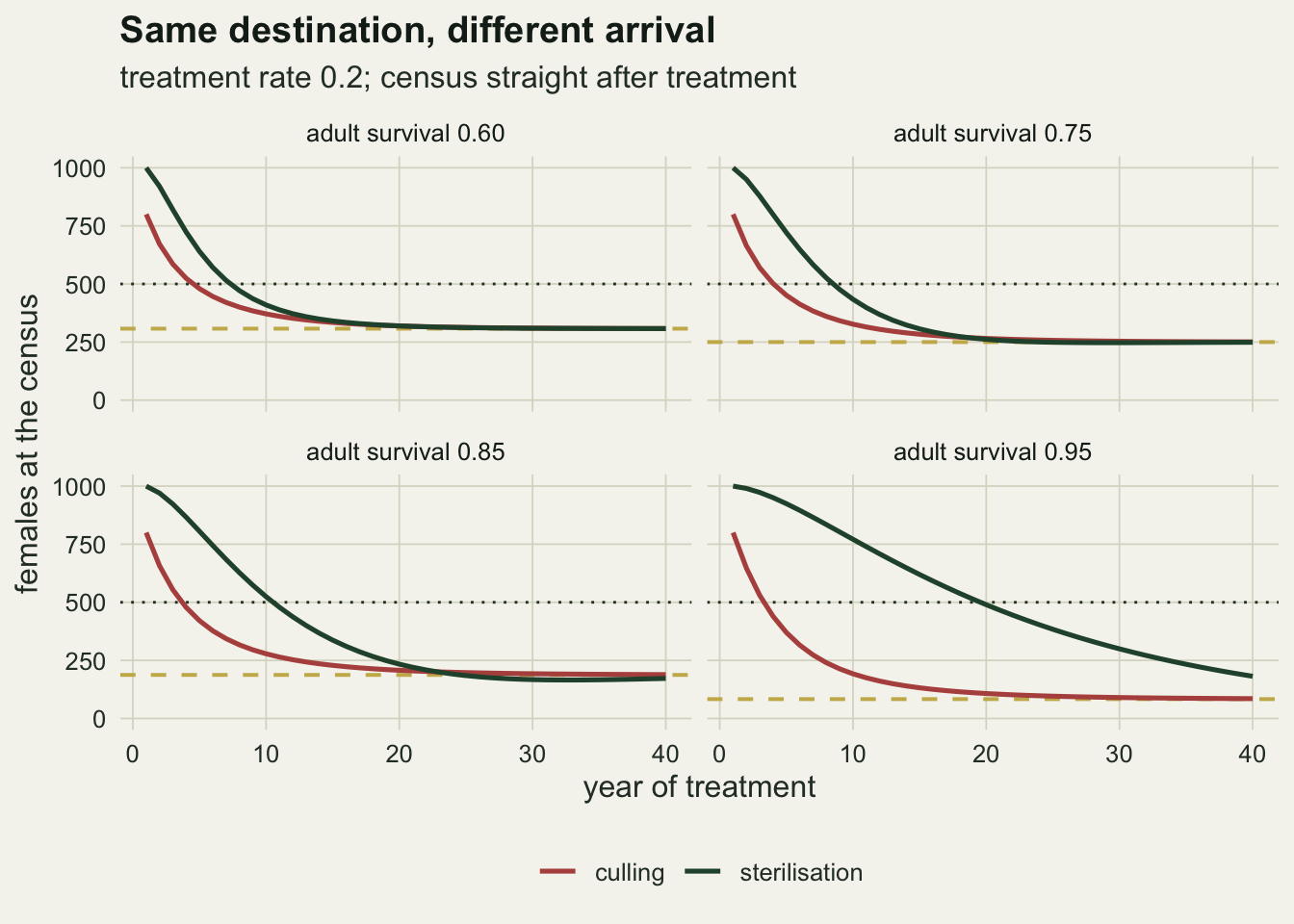
A map of the lag
map_grid <- expand.grid(s_a = seq(0.50, 0.95, by = 0.01), h = seq(0.02, 0.50, by = 0.01))
n_map    <- 150
map_grid$t_cull <- first_below(project(map_grid$s_a, map_grid$h, n_map, "cull")$pop)
map_grid$t_ster <- first_below(project(map_grid$s_a, map_grid$h, n_map, "sterile")$pop)
map_grid$lag    <- map_grid$t_ster - map_grid$t_cull
map_grid$eq     <- p_star(map_grid$s_a, map_grid$h)

reach    <- !is.na(map_grid$lag)
n_reach  <- sum(reach)
n_cells  <- nrow(map_grid)
n_nonpos <- sum(map_grid$lag[reach] <= 0)
eq_nonpos_min <- min(map_grid$eq[reach & map_grid$lag <= 0])
lag_max  <- max(map_grid$lag[reach])
at_max   <- map_grid[reach & map_grid$lag == lag_max, ][1, ]
lag_hi_crit <- map_grid$lag[reach & abs(map_grid$s_a - 0.95) < 1e-9 & abs(map_grid$h - 0.30) < 1e-9]
lag_lo_crit <- map_grid$lag[reach & abs(map_grid$s_a - 0.60) < 1e-9 & abs(map_grid$h - 0.30) < 1e-9]
row_95   <- map_grid$lag[reach & abs(map_grid$s_a - 0.95) < 1e-9]
row_60   <- map_grid$lag[reach & abs(map_grid$s_a - 0.60) < 1e-9]
miss      <- !reach
n_miss_eq <- sum(miss & map_grid$eq > half_pop + 1e-6 & is.na(map_grid$t_ster))
n_only_s  <- sum(miss & is.na(map_grid$t_cull) & !is.na(map_grid$t_ster))
n_on_line <- sum(miss & abs(map_grid$eq - half_pop) < 1e-6)
n_tie     <- sum(map_grid$lag[reach] == 0)

# the same four life histories with the treatment rate chosen so that the
# shared equilibrium is 200 females in every case
h_match <- sapply(s_show, function(s_val)
  uniroot(function(h) p_star(s_val, h) - 200, c(1e-4, h_crit - 1e-6), tol = 1e-10)$root)
lag_match <- first_below(project(s_show, h_match, 300, "sterile")$pop) -
  first_below(project(s_show, h_match, 300, "cull")$pop)
Over a grid of 2254 combinations, a 50 per cent reduction is reached within 150 years in 1824 of them under both levers. Of the rest, 426 have an equilibrium above half the starting population and neither lever gets there; in 4 sterilisation dips under the line while culling, which approaches its equilibrium from above, never does, and 3 of those have an equilibrium lying on the 500 line itself. Where it is reached, the largest lag is 21 years, at adult survival 0.95 and treatment rate 0.05. At a treatment rate of 0.3 the lag is 2 years at adult survival 0.60 and 16 years at 0.95. Holding survival at 0.95 and moving the treatment rate across its reachable range, the lag runs from 14 to 21 years; at survival 0.60 it runs from 2 to 3.
Because the design ties the density coefficient to survival, the equilibrium at a fixed rate is deeper for long-lived species, and some of the growth in the lag could be a depth effect. Choosing the treatment rate for each life history so that the shared equilibrium is 200 females (rates of 0.242, 0.222, 0.194 and 0.118) gives lags of 2, 4, 7 and 18 years, so the lag still grows with survival at a matched end point.
In 8 cells sterilisation reaches the target no later than culling, and 5 of those are ties. All of them sit along the edge of the reachable region, with an equilibrium of at least 491 females, where both populations creep towards a line they only just cross; in the few that are not ties the slightly oscillating sterile trajectory dips under it first. They are an artefact of a fixed target near an equilibrium, not an advantage of the lever.
ggplot(map_grid, aes(s_a, h, fill = lag)) +
  geom_raster() +
  geom_hline(yintercept = h_crit, linetype = "dashed", colour = te_ink,
             linewidth = 0.6) +
  scale_fill_gradient(low = te_gold, high = te_forest, na.value = te_line,
                      name = "lag, years") +
  scale_x_continuous(expand = c(0, 0)) +
  scale_y_continuous(expand = c(0, 0)) +
  labs(x = "adult survival", y = "annual treatment rate",
       title = "The lag grows with survival",
       subtitle = "years to a 50 per cent reduction, sterilisation minus culling") +
  theme_datasheet() +
  theme(legend.position = "right")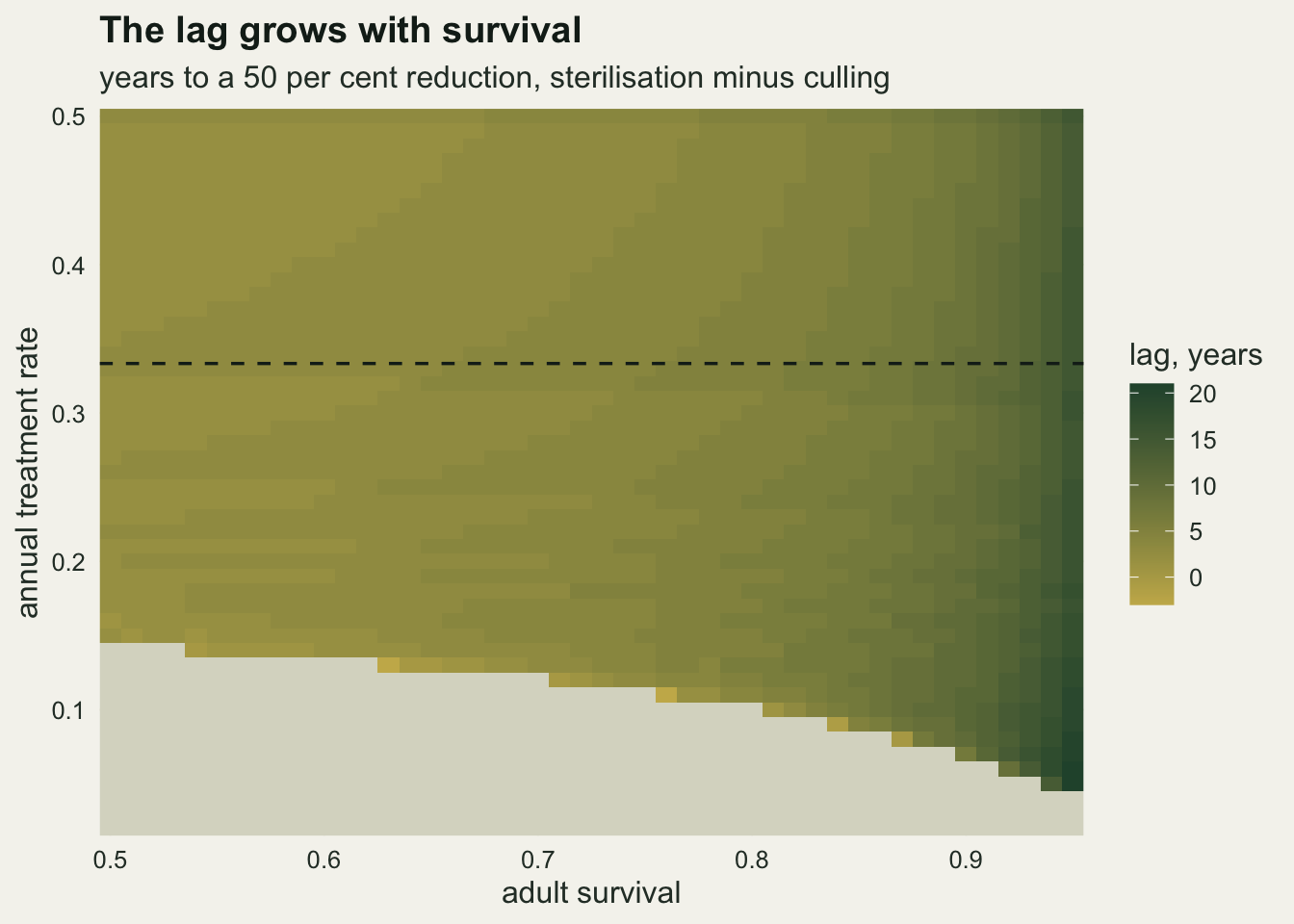
Animals handled: fewer a year, more to the target
n_hand <- 40
hand_c <- project(s_show, 0.2, n_hand, "cull")$hand
hand_s <- project(s_show, 0.2, n_hand, "sterile")$hand
to_half_c <- hand_c[cbind(1:4, t50_c)]
to_half_s <- hand_s[cbind(1:4, t50_s)]
yearly_c <- t(apply(hand_c, 1, diff))
yearly_s <- t(apply(hand_s, 1, diff))
n_less   <- sum(yearly_s < yearly_c)
n_pairs  <- length(yearly_c)

annual_c <- 0.2 * eq_02 / (1 - 0.2)
annual_s <- 0.2 * f_star(s_show, 0.2) / (1 - 0.2)
In the first year both teams handle the same 200 females. After that the darting team handles fewer each year: over years 2 to 40 and the four life histories, its yearly count is the smaller one in 156 of 156 comparisons. Handling is the treatment rate times the untreated females, and under sterilisation part of the census is already sterile and holds down recruitment, so fewer untreated females appear. At the shared equilibrium culling handles 46.9 females a year and sterilisation 17.6 at adult survival 0.85; at 0.95 the figures are 20.8 and 3.5.
The target is a different matter, because sterilisation needs more years to get there. Up to the year the population is halved at a treatment rate of 0.2, the darting team handles 917 to 1005 females across the four life histories, and the marksman team 604 to 765. Which lever is cheaper in handling depends on whether the bill is counted to the target or over the life of the programme, and an argument about cost that does not say which is not yet about cost.
keep <- c(1, 4)
hand_df <- rbind(
  data.frame(year = rep(seq_len(n_hand), each = 2), s_a = rep(s_show[keep], n_hand),
             handled = as.vector(hand_c[keep, ]), lever = "culling"),
  data.frame(year = rep(seq_len(n_hand), each = 2), s_a = rep(s_show[keep], n_hand),
             handled = as.vector(hand_s[keep, ]), lever = "sterilisation"))
hand_df$panel <- factor(sprintf("adult survival %.2f", hand_df$s_a))
mark_df <- data.frame(
  year = c(t50_c[keep], t50_s[keep]),
  handled = c(to_half_c[keep], to_half_s[keep]),
  lever = rep(c("culling", "sterilisation"), each = 2),
  panel = factor(sprintf("adult survival %.2f", rep(s_show[keep], 2))))

ggplot(hand_df, aes(year, handled, colour = lever)) +
  geom_line(linewidth = 0.9) +
  geom_point(data = mark_df, size = 2.6) +
  facet_wrap(~ panel) +
  scale_colour_manual(values = c(culling = te_rust, sterilisation = te_forest),
                      name = NULL) +
  labs(x = "year of treatment", y = "females handled, cumulative",
       title = "Fewer a year, more to the target",
       subtitle = "treatment rate 0.2; points: the year of a 50 per cent reduction") +
  theme_datasheet() +
  theme(legend.position = "bottom",
        strip.text = element_text(colour = te_ink))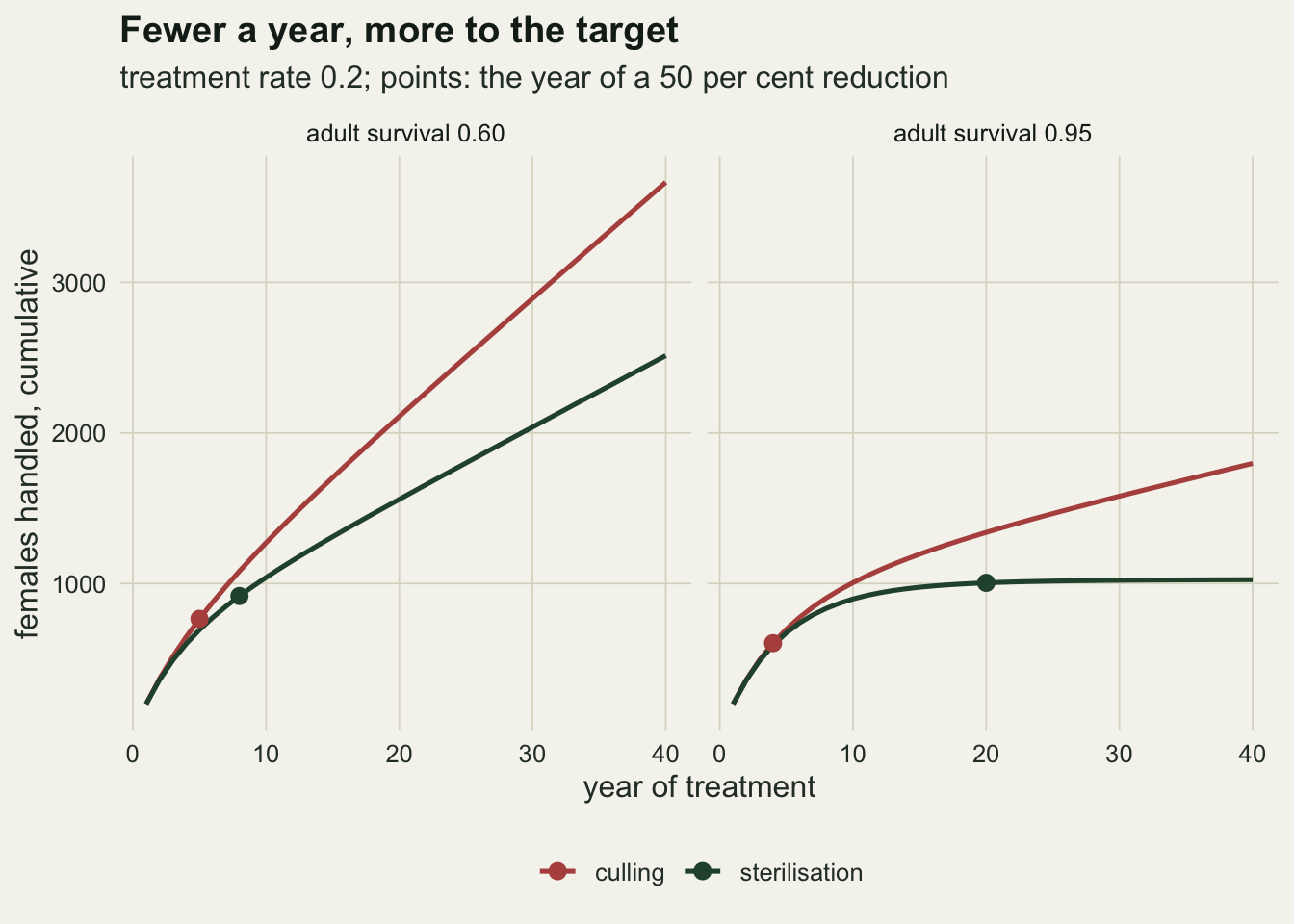
The census point is part of the identity
pre_ratio <- 1 / (1 - 0.2)
pre_cull_85 <- eq_02[3] * pre_ratio

# counted before treatment: the culled count is pop / (1 - h), the sterile count
# does not change because treatment moves animals between classes
t50_c_pre <- first_below(traj_c$pop / (1 - 0.2))
lag_pre   <- t50_s - t50_c_pre
lag_post  <- t50_s - t50_c
The equality of end points holds for a census taken after the treatment. Count before it instead, and a culled population at equilibrium is 1.25 times the post-treatment count at a treatment rate of 0.2, because the animals about to be shot are still standing there; at adult survival 0.85 that is 234.4 females against 187.5. The sterilised count does not change, because treatment removes nothing. Two reports that compare the levers with counts from different sides of the treatment will find a difference the populations do not have. Matrix population models draw the same distinction between a census taken before and after breeding (Caswell 2001), and the choice changes what a count means. The density effect in the model acts on the animals present in the breeding season, which is the post-treatment count; that choice and the census choice have to be stated together.
The lag moves too. Counted before treatment, culling halves the population in 9, 7, 6 and 5 years at adult survival 0.60, 0.75, 0.85 and 0.95, so the lag is -1, 2, 5 and 15 years instead of 3, 4, 7 and 16. At adult survival 0.60 sterilisation now gets there first: on the post-treatment count the first year’s cull is booked at once, and that head start is bookkeeping, not biology. This post uses the post-treatment count because it is the number of animals living in the reserve through the year, the number the density feedback sees, and the count on which the two end points are identical. The growth of the lag with survival survives the change of census; its size, and at low survival its sign, do not.
Demographic noise at the bottom
The deterministic recursion carries fractions of a deer. With binomial treatment and survival and Poisson recruitment, 300 runs per setting over 60 years show how much the timing wobbles and what happens once the equilibrium is small.
n_run  <- 300
n_dem  <- 60
set.seed(20904)
dem_rows <- list()
for (h_val in c(0.2, 0.3)) for (s_val in s_show) for (lv in c("cull", "sterile")) {
  sim <- project(s_val, rep(h_val, n_run), n_dem, lv, demographic = TRUE)
  t50 <- first_below(sim$pop)
  dem_rows[[length(dem_rows) + 1]] <- data.frame(
    h = h_val, s_a = s_val, lever = ifelse(lv == "cull", "culling", "sterilisation"),
    t50_med = median(t50, na.rm = TRUE),
    t50_lo  = unname(quantile(t50, 0.05, na.rm = TRUE)),
    t50_hi  = unname(quantile(t50, 0.95, na.rm = TRUE)),
    n_miss  = sum(is.na(t50)),
    below10 = mean(apply(sim$pop, 1, min) < 10),
    no_fert = mean(sim$fert[, n_dem] == 0),
    pop_end = median(sim$pop[, n_dem]))
}
dem <- do.call(rbind, dem_rows)
dem$no_fert_se <- sqrt(dem$no_fert * (1 - dem$no_fert) / n_run)
pick <- function(h_val, s_val, lv, col) dem[dem$h == h_val & abs(dem$s_a - s_val) < 1e-9 & dem$lever == lv, col]
f_eq_95 <- f_star(0.95, 0.2)
f_eq_85_3 <- f_star(0.85, 0.3)
lost_rows <- dem[dem$lever == "sterilisation" & dem$no_fert > 0.05, ]
eq_lost_max <- max(p_star(lost_rows$s_a, lost_rows$h))
n_lost <- nrow(lost_rows)
n_cull_lost <- sum(dem$lever == "culling" & dem$no_fert > 0.05)
red_lost <- 1 - eq_lost_max / k_cap

# deterministic fertile trough under sterilisation, over the same 60 years
det_f95  <- project(0.95, 0.2, n_dem, "sterile")$fert[1, ]
det_f853 <- project(0.85, 0.3, n_dem, "sterile")$fert[1, ]
min_f95 <- min(det_f95); yr_f95 <- which.min(det_f95)
min_f853 <- min(det_f853); yr_f853 <- which.min(det_f853)
At a treatment rate of 0.2 the timing barely moves: the 90 per cent range of the year of halving is 4 to 4 for culling and 19 to 22 for sterilisation at adult survival 0.95, against deterministic values of 4 and 20. Starting from 1000 females, demographic noise does not blur the lag.
It does change the bottom, and the reason starts in the deterministic run. At adult survival 0.95 and a rate of 0.2 the sterilisation equilibrium would hold 13.9 fertile females inside a census of 83.3, but the deterministic run never gets near that value within 60 years: it carries only 0.46 fertile females in year 56. The sterile animals keep recruitment suppressed while the fertile class is treated away, so the fertile count undershoots its equilibrium far further than the census does. A fraction of a female is not a female, and with demographic noise that trough becomes permanent: by year 60 no fertile female is left in 0.907 of the runs (Monte Carlo standard error 0.017), against 0.000 under culling. The median census there is still 65 females, and in the runs that lost the breeding core all of them are sterile and ageing out. At a rate of 0.3 and survival 0.85 the fertile equilibrium is 9.6 females and the deterministic trough 5.9 in year 32; the trough stays above one female, and noise alone takes the breeding group by year 60 in 0.620 of sterilisation runs, against 0.013 of culling runs. The culled census cannot undershoot in this way, because its recursion approaches the equilibrium from one side.
So the equal end point is a statement about the census total. Because sterilisation stores part of that total in animals that cannot breed, and at high survival most of it, its breeding core is smaller at the same census and passes through a deeper trough on the way, and demographic noise can finish it off where culling leaves a small breeding population in place. That is a real difference, but a narrow one. Of the 8 sterilisation settings run, 5 lost the breeding core in more than five per cent of runs (1 of the culling settings did), and every one of them has a shared equilibrium of at most 83.3 females, a reduction of more than 91 per cent. It is not an argument that sterilisation is generally stronger, and the deterministic identity was never meant to cover a population that small.
dem02 <- dem[dem$h == 0.2, ]
p_time <- ggplot(dem02, aes(s_a, t50_med, colour = lever)) +
  geom_errorbar(aes(ymin = t50_lo, ymax = t50_hi), width = 0.015, linewidth = 0.6) +
  geom_point(size = 2.4) +
  scale_colour_manual(values = c(culling = te_rust, sterilisation = te_forest),
                      name = NULL) +
  scale_x_continuous(breaks = s_show) +
  labs(x = "adult survival", y = "year of 50 per cent reduction",
       title = "Timing") +
  theme_datasheet() +
  theme(legend.position = "none")
dem$rate <- factor(sprintf("rate %.1f", dem$h))
p_fert <- ggplot(dem, aes(s_a, no_fert, colour = lever, linetype = rate)) +
  geom_line(linewidth = 0.8) +
  geom_point(size = 2) +
  scale_colour_manual(values = c(culling = te_rust, sterilisation = te_forest),
                      name = NULL) +
  scale_linetype_manual(values = c("dashed", "solid"), name = NULL) +
  scale_x_continuous(breaks = s_show) +
  scale_y_continuous(limits = c(0, 1)) +
  labs(x = "adult survival", y = "share of runs, no fertile female",
       title = "Breeding core lost by year 60") +
  guides(colour = guide_legend(nrow = 2), linetype = guide_legend(nrow = 2)) +
  theme_datasheet() +
  theme(legend.position = "bottom")
(p_time | p_fert) +
  plot_annotation(theme = theme_datasheet())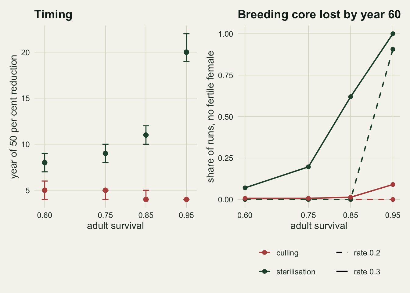
Which assumptions make the answer different
The identity rests on one line of the derivation: the fertile multiplier depends on the census total, and the census total is the same object under both levers. Three changes to the treated animals were set before running, at adult survival 0.85 and a treatment rate of 0.2, and each one touches a different part of that line.
s_v <- 0.85; h_v <- 0.2; n_v <- 2000
dm_v <- demog(s_v); bonus_v <- 0.05
runs_v <- list(
  culling        = project(s_v, h_v, n_v, "cull"),
  sterilisation  = project(s_v, h_v, n_v, "sterile"),
  outside        = project(s_v, h_v, n_v, "sterile", sterile_in_dd = FALSE),
  bonus          = project(s_v, h_v, n_v, "sterile", bonus = bonus_v),
  season         = project(s_v, h_v, n_v, "season"))
end_v   <- sapply(runs_v, function(x) x$pop[n_v])
t50_v   <- sapply(runs_v, function(x) first_below(x$pop))
yr_v    <- sapply(runs_v, function(x) x$hand[n_v] - x$hand[n_v - 1])

closed_v <- c(
  culling       = p_star(s_v, h_v),
  sterilisation = p_star(s_v, h_v),
  outside       = p_star(s_v, h_v) * (1 + h_v / ((1 - h_v) * (1 - s_v))),
  bonus         = p_star(s_v, h_v),
  season        = (dm_v$r0 * (1 - h_v) / (1 - s_v) - 1) / dm_v$cc)
gap_v    <- max(abs(end_v - closed_v))
h_season <- 1 - (1 - s_v) / dm_v$r0
fert_bonus <- runs_v$bonus$fert[n_v]
fert_base  <- runs_v$sterilisation$fert[n_v]
Sterile animals left out of the density feedback, for example because they no longer lactate and eat less in the limiting season, break the identity at its root. The fertile multiplier now sees only fertile females, so the fertile equilibrium takes the old census value and the sterile animals are added on top: the long-run census is 500.0 females against 187.5 under culling, which with these constants lands on the 50 per cent line itself (a coincidence of adult survival 0.85 and a rate of 0.2), so the target is approached but not crossed. The annual handling is 46.9 females, the same as culling, for a population 2.67 times larger.
A survival bonus for treated females, 0.05 added to adult survival, does not move the census end point at all, and the closed form says why: the equilibrium condition involves only the fertile multiplier and the census total, not the fate of the sterile animals. It settles at 187.5 females, as without the bonus. What it changes is the split and the speed: 53.6 fertile females at equilibrium instead of 70.3, and 14 years to halve the population instead of 11. Longer-lived sterile animals make the lever slower here, not different.
A contraceptive that works for one breeding season only turns the lever into a different one. Treated females still survive at the adult rate and only their recruitment is lost, so the treatment no longer cuts into the survival term of the multiplier. The long-run census is 740.0 females, the handling needed each year is 148.0, and driving the population to extinction needs a rate above 0.769, against 0.333 for culling. Across the five versions the simulated end points match their closed forms to within 7.39e-13 animals.
n_vs <- 60
lab_v <- c(culling = "culling", sterilisation = "sterilisation",
           outside = "sterile animals outside density feedback",
           bonus = "sterile females survive 0.05 better",
           season = "contraceptive lasts one season")
var_df <- do.call(rbind, lapply(names(runs_v), function(nm)
  data.frame(year = seq_len(n_vs), pop = runs_v[[nm]]$pop[1, seq_len(n_vs)],
             version = lab_v[[nm]])))
var_df$version <- factor(var_df$version, levels = unname(lab_v))

ggplot(var_df, aes(year, pop, colour = version, linetype = version)) +
  geom_hline(yintercept = half_pop, linetype = "dotted", colour = te_body,
             linewidth = 0.5) +
  geom_line(linewidth = 0.9) +
  scale_colour_manual(values = c(te_rust, te_forest, te_gold, te_forest, te_ink),
                      name = NULL) +
  scale_linetype_manual(values = c("solid", "solid", "solid", "dashed", "solid"),
                        name = NULL) +
  scale_y_continuous(limits = c(0, k_cap)) +
  labs(x = "year of treatment", y = "females at the census",
       title = "Slower or different",
       subtitle = "adult survival 0.85, treatment rate 0.2") +
  guides(colour = guide_legend(ncol = 2), linetype = guide_legend(ncol = 2)) +
  theme_datasheet() +
  theme(legend.position = "bottom")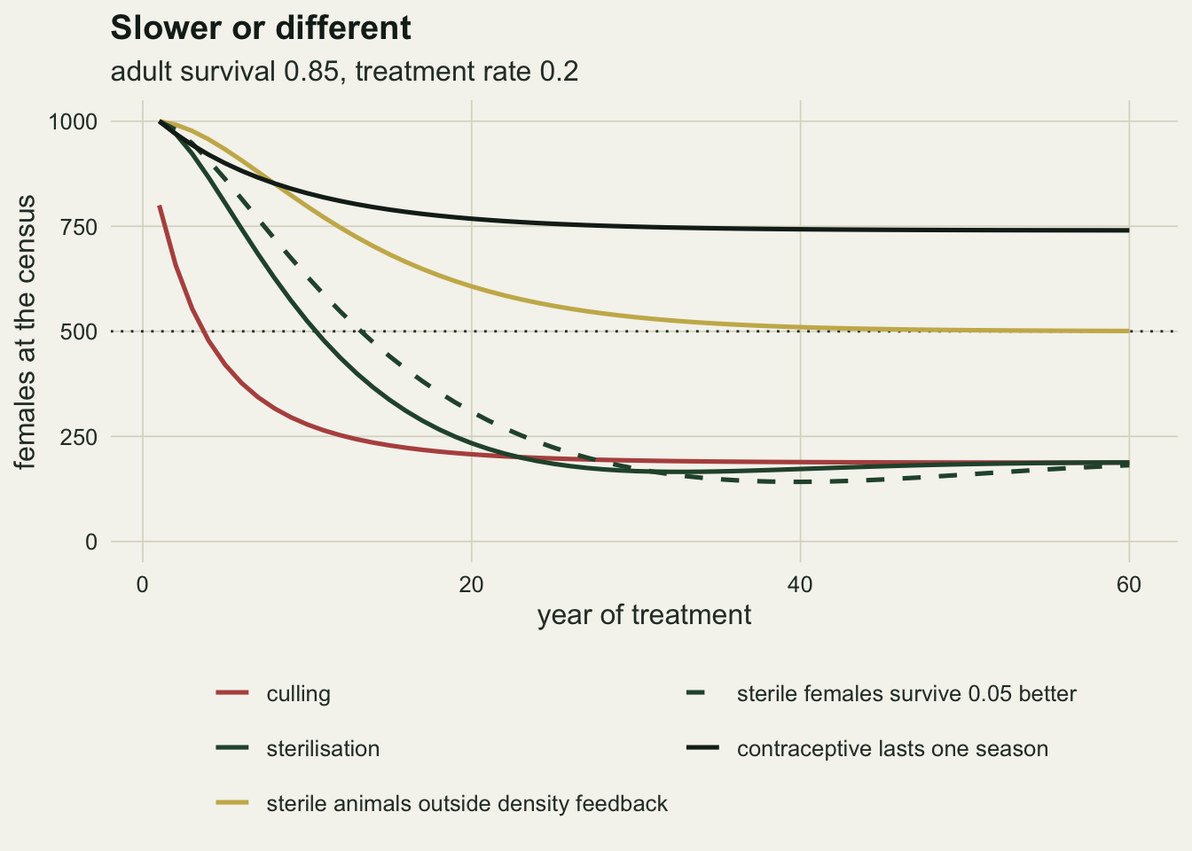
What to report
State the census point, and state it relative to the treatment. A comparison of culling and fertility control that counts before a cull and after a sterilisation measures the calendar, not the levers. The census point moves the lag as well as the end point.
State which animals the density feedback counts. With sterile animals in it, the two levers at the same treatment rate share a long-run census and differ in time; with sterile animals outside it, they differ in the end point. This is a biological claim about the species and the limiting resource, and the model result is only as good as that claim.
Report time and handling together, with a horizon. Sterilisation handles fewer animals a year but, except at low survival on a count taken before treatment, needs more years to reach a reduction target, and on the post-treatment count more handled animals in total; both statements are true at once. For a long-lived species the lag is the number to put in front of a committee, because a ten year evaluation of a sterilisation programme can look like failure when the census is on schedule. At high survival, check the fertile count as well as the census: the programme can be on schedule to lose its breeding core rather than to settle at the target.
Say whether the contraceptive is permanent. A one-season product is not a slower version of sterilisation but a separate lever with its own critical rate, and the rates measured for a permanent sterilant do not carry over to it.
Honest limits
The model is females only: recruits join the breeding class at the next census, and there is no age structure, no male side (Barlow and colleagues found that the mating system changes the efficacy of sterilisation, which a females-only model cannot see), no immigration and no environmental noise. Immigration is the omission most likely to matter in a suburban reserve, because culled space can be refilled from outside while sterile residents keep occupying theirs; how that plays out depends on territorial behaviour that is not in the model, and a reserve with a leaky boundary needs a spatial model before either lever is compared.
The maximum annual multiplier of 1.5 and the untreated equilibrium of 1000 were fixed across life histories, which ties recruitment to survival. With recruitment held constant instead, the critical rate would rise with survival and part of the survival effect above would be a distance-to-critical-rate effect. The mechanism of the lag, sterile animals persisting for an expected one over one minus survival years, is not tied to that choice, and the matched-equilibrium check shows the lag still growing with survival when the end point is held fixed; but no run here redraws the lag map with recruitment held constant, and none of its numbers should be carried over.
Treatment is perfect and instantaneous, and handling is counted in animals, not in money. Darting a wary female twice for a booster, locating unmarked females in a large herd, and the fact that sterile animals must be identifiable to avoid re-treatment all change the effort ledger, and a real cost comparison needs costs per animal for each lever.
The target of a 50 per cent reduction is a fixed line, and near the edge of the reachable region the years to cross it are sensitive to small, slow oscillations. The handful of cells where sterilisation crosses first, or where only sterilisation crosses, come from that sensitivity. A target defined as a share of the distance to equilibrium would remove the edge effect but is not how reduction targets are written.
The demographic noise is binomial and Poisson around the deterministic rates. The loss of the breeding core under sterilisation depends on how deep the deterministic fertile trough runs and how small the fertile equilibrium is. Year-to-year variation in recruitment is not in the model, and nothing here says which lever is more at risk once it is added.
References
Hobbs NT, Bowden DC, Baker DL 2000 Journal of Wildlife Management 64(2):473-491 (10.2307/3803245)
Barlow ND, Kean JM, Briggs CJ 1997 Wildlife Research 24(2):129-141 (10.1071/WR95027)
Caswell H 2001 Matrix Population Models, 2nd ed, Sinauer Associates (ISBN 978-0-87893-096-8)