---
title: "Leslie matrix population models in R"
description: "Turn a life table into a Leslie matrix in R and read growth rate, stable age distribution and reproductive value from its dominant eigenvalue and eigenvectors."
date: 2026-07-05 10:00
categories: [R, population dynamics, demography, matrix models, ecology tutorial]
image: thumbnail.png
image-alt: "Bar chart of the stable age distribution from a Leslie matrix, declining across five age classes"
---
A life table gives you a growth rate, but a Leslie matrix gives you more: the same growth rate as a matrix eigenvalue, plus the age structure the population settles into and the reproductive value of each age. This post builds a Leslie matrix from the demography of the [previous post](../life-tables-and-lambda/), confirms its dominant eigenvalue equals the `lambda` from the Euler-Lotka equation, and reads the stable age distribution and reproductive value directly off the eigenvectors. It also shows the single most common construction mistake, which inflates the growth rate by nearly a third.
## Building the matrix
A Leslie matrix projects an age-structured population one step forward: multiply the vector of counts by age by the matrix, and you get next year's counts. The structure is fixed. Survivals sit on the subdiagonal, moving individuals from one age to the next, and fertilities sit in the top row, sending new offspring into the first class. The one part that trips people up is the fertility coefficient.
```{r}
#| label: setup
#| message: false
#| warning: false
library(ggplot2)
library(dplyr)
library(tidyr)

te_ink <- "#16241d"; te_forest <- "#275139"; te_gold <- "#c9b458"
te_faint <- "#5d6b61"; te_line <- "#dad9ca"; te_paper <- "#f5f4ee"
theme_te <- function(base_size = 12) {
  theme_minimal(base_size = base_size) +
    theme(text = element_text(colour = "#2c3a31"),
          plot.title = element_text(colour = te_ink, face = "bold", size = base_size * 1.15),
          plot.subtitle = element_text(colour = te_faint, size = base_size * 0.95),
          axis.title = element_text(colour = "#46604a"), axis.text = element_text(colour = te_faint),
          panel.grid.minor = element_blank(),
          panel.grid.major = element_line(colour = te_line, linewidth = 0.3),
          plot.background = element_rect(fill = te_paper, colour = NA),
          panel.background = element_rect(fill = te_paper, colour = NA),
          legend.key = element_rect(fill = te_paper, colour = NA),
          strip.text = element_text(colour = te_ink, face = "bold"))
}

## same demography as the life-table post; census just before breeding,
## so newborns first appear at age 1 (ages 1 to 5 are the matrix classes)
p0        <- 0.50                          # first-year survival (age 0 to 1)
surv_1to5 <- c(0.60, 0.70, 0.70, 0.50)     # survival age 1->2, 2->3, 3->4, 4->5
m_age     <- c(0.00, 1.50, 2.00, 1.70, 1.00)  # fecundity at ages 1 to 5

Fi <- p0 * m_age                            # pre-breeding fertility coefficient
L  <- matrix(0, 5, 5)
L[1, ] <- Fi
for (i in 1:4) L[i + 1, i] <- surv_1to5[i]
L
```
The top row is `p0 * m_age`, not `m_age`. In a census taken just before breeding, a female of age `i` produces `m_age[i]` offspring, but those offspring are not counted until they survive their first year and reach age 1. The factor `p0` carries them there. Skipping it is the classic error.
```{r}
#| label: naive-vs-correct
L_naive <- L
L_naive[1, ] <- m_age                       # fertility without first-year survival
lam_correct <- Re(eigen(L)$values[1])
lam_naive   <- Re(eigen(L_naive)$values[1])
c(correct = lam_correct, naive = lam_naive,
  overestimate_pct = 100 * (lam_naive - lam_correct) / lam_correct)
```
Forgetting the first-year survival treats every newborn as if it instantly became a counted yearling. Here that overstates the growth rate by twenty-eight percent, turning a population that grows six percent a year into one that appears to grow thirty-six percent a year. The size of the error scales with how low first-year survival is.
## The dominant eigenvalue is the growth rate
The correct dominant eigenvalue is about 1.0622, exactly the `lambda` the Euler-Lotka equation returned for the same demography. That is not a coincidence: the characteristic polynomial of a Leslie matrix is the discrete Euler-Lotka equation. The matrix and the life table are two descriptions of one process.
```{r}
#| label: eigenvalue
ev  <- eigen(L)
lam <- Re(ev$values[1])
lam2 <- sort(Mod(ev$values), decreasing = TRUE)[2]
c(lambda = lam, second_eigenvalue = lam2)
```
The second eigenvalue, about 0.54, controls how fast the population converges to its stable structure: the further it sits below the dominant eigenvalue, the quicker the transients fade. That ratio is the subject of transient analysis, beyond this post.
## Projecting the population
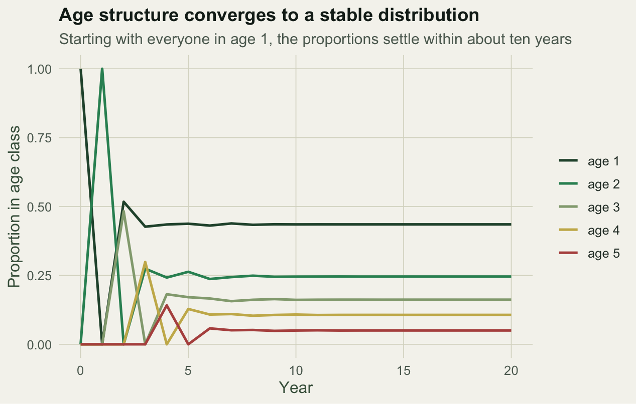
To see the matrix work, start a population entirely in the first age class and project it forward. Two things happen. The total settles into geometric growth at rate `lambda`, and the age proportions settle into a fixed distribution regardless of where they started.
```{r}
#| label: projection
n0 <- c(100, 0, 0, 0, 0)
steps <- 20
N <- matrix(0, steps + 1, 5); N[1, ] <- n0
for (t in 1:steps) N[t + 1, ] <- as.numeric(L %*% N[t, ])

total <- rowSums(N)
ratio <- total[-1] / total[-length(total)]
c(ratio_year1 = ratio[1], ratio_year10 = ratio[10], ratio_year20 = ratio[20], lambda = lam)
```
The year-on-year ratio starts at 0.60, because the first cohort is all yearlings that do not yet breed and simply survive to age 2, then climbs and settles on `lambda`. The early wobble is the transient; the long-run rate is the eigenvalue.
```{r}
#| label: fig-convergence
#| fig-cap: "Age proportions converge to a stable distribution within about ten years."
#| fig-alt: "Five lines showing the proportion of the population in each age class over twenty years; starting spread out, they converge to steady values by year ten."
#| fig-width: 6.6
#| fig-height: 4.2
prop <- N / rowSums(N)
pd <- as.data.frame(prop); colnames(pd) <- paste("age", 1:5); pd$year <- 0:steps
pd_long <- pivot_longer(pd, starts_with("age"), names_to = "class", values_to = "prop")
ggplot(pd_long, aes(year, prop, colour = class)) +
  geom_line(linewidth = 0.9) +
  scale_colour_manual(values = c("#275139", "#2f8f63", "#93a87f", "#c9b458", "#b5534e"),
                      name = NULL) +
  labs(title = "Age structure converges to a stable distribution",
       subtitle = "Starting with everyone in age 1, the proportions settle within about ten years",
       x = "Year", y = "Proportion in age class") +
  theme_te()
```
## Stable age distribution and reproductive value
The distribution the proportions converge to is the right eigenvector of the matrix, scaled to sum to one. It says what fraction of a population at its stable structure sits in each age class.
```{r}
#| label: stable-distribution
w <- Re(ev$vectors[, 1]); w <- w / sum(w)
round(100 * w, 1)
```
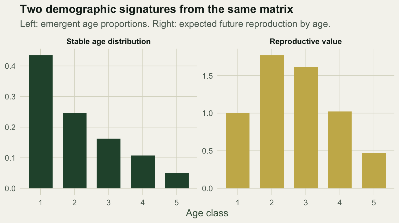
At the stable structure about forty-four percent of individuals are yearlings and the fraction falls steadily with age, the shape you expect from steep early mortality. The left eigenvector carries the complementary information: reproductive value, the expected contribution of an individual of each age to future population growth.
```{r}
#| label: reproductive-value
vleft <- Re(eigen(t(L))$vectors[, 1])
vleft <- vleft / vleft[1]                    # scale so age 1 has value 1
round(vleft, 3)
```
Reproductive value peaks at age 2, the age of first reproduction, then declines as an individual's remaining reproduction shrinks. A yearling has value 1 by convention; a two-year-old is worth about 1.77 yearlings because it has survived the risky early period and is about to reproduce. Reproductive value is why conservation often prioritises breeding-age adults over eggs or juveniles.
```{r}
#| label: fig-signatures
#| fig-cap: "Stable age distribution and reproductive value, the right and left eigenvectors."
#| fig-alt: "Two bar charts: the left declines across age classes (stable age distribution), the right rises to a peak at age two then declines (reproductive value)."
#| fig-width: 6.8
#| fig-height: 3.8
sig <- data.frame(age = factor(1:5), stable = w, rv = vleft) |>
  pivot_longer(c(stable, rv), names_to = "quantity", values_to = "value")
sig$quantity <- factor(sig$quantity, levels = c("stable", "rv"),
                       labels = c("Stable age distribution", "Reproductive value"))
ggplot(sig, aes(age, value, fill = quantity)) +
  geom_col(width = 0.7, show.legend = FALSE) +
  facet_wrap(~quantity, scales = "free_y") +
  scale_fill_manual(values = c(te_forest, te_gold)) +
  labs(title = "Two demographic signatures from the same matrix",
       subtitle = "Left: emergent age proportions. Right: expected future reproduction by age.",
       x = "Age class", y = NULL) +
  theme_te()
```
## What to take away
A Leslie matrix packs a life table into a form whose eigenstructure answers three questions at once. The dominant eigenvalue is the asymptotic growth rate, identical to the Euler-Lotka `lambda`. The right eigenvector is the stable age distribution. The left eigenvector is reproductive value. Build the top row as survival times fecundity, not fecundity alone, or the growth rate comes out badly wrong. The natural next question, which matrix entry most changes `lambda`, is what sensitivity and elasticity analysis answers.
## References
- Leslie PH 1945 Biometrika 33(3):183-212 (10.1093/biomet/33.3.183)
- Leslie PH 1948 Biometrika 35(3-4):213-245 (10.1093/biomet/35.3-4.213)
- Fisher RA 1930 The Genetical Theory of Natural Selection, Clarendon Press, Oxford (pre-ISBN)
- Caswell H 2001 Matrix Population Models, 2nd ed, Sinauer Associates (ISBN 978-0-87893-096-8)
- Gotelli NJ 2008 A Primer of Ecology, 4th ed, Sinauer Associates (ISBN 978-0-87893-318-1)
## Related tutorials
- [Life tables and population growth in R](../life-tables-and-lambda/)
- [Stage-structured Lefkovitch matrices in R](../stage-structured-lefkovitch/)
- [Sensitivity and elasticity of matrix models](../matrix-sensitivity-elasticity/)