library(ggplot2)
library(dplyr)
library(tidyr)Transient dynamics of population matrix models
R
population dynamics
matrix models
transient dynamics
ecology tutorial
Compute the transient indices of a stage-structured matrix in R: reactivity, amplification and the damping ratio, and see why the initial structure matters.
The dominant eigenvalue of a projection matrix tells you the long-run growth rate, but a population reaches that rate only after its stage structure settles onto the stable distribution. Until then it behaves differently, sometimes dramatically so: a stand of all mature plants can boom for a few years before slowing, while a cohort of all seedlings can crash before recovering. These short-term departures are the transient dynamics, and for a population that is disturbed, reintroduced or harvested, they can matter more than the asymptotic rate. This post computes the standard transient indices in base R, reactivity, amplification and the damping ratio, and shows how the starting structure sets the near-term path.
A stage-structured matrix
The example is a long-lived perennial with four stages: seedling, juvenile, small adult and large adult. Large adults survive well and are the main reproducers, so the matrix mixes slow growth with high adult stasis.
A <- matrix(c(0,    0,    0.40, 1.80,
              0.20, 0.35, 0,    0,
              0,    0.40, 0.55, 0,
              0,    0,    0.35, 0.90), nrow = 4, byrow = TRUE)
stages <- c("Seedling", "Juvenile", "Small adult", "Large adult")

ev <- eigen(A)
ord <- order(Mod(ev$values), decreasing = TRUE)
lambda1 <- Re(ev$values[ord[1]])
lambda2 <- ev$values[ord[2]]
damping <- lambda1 / Mod(lambda2)
c(lambda1 = lambda1, mod_lambda2 = Mod(lambda2), damping_ratio = damping)
lambda1 mod_lambda2 damping_ratio
1.0501299 0.5257223 1.9974993 The asymptotic growth rate is about 1.05, a population increasing near 5 percent per year. The damping ratio, the dominant eigenvalue divided by the modulus of the subdominant one, is about 2.0. That number controls how fast the transient fades: the distance to the stable structure shrinks by roughly a factor of two each year.
Stable structure and reproductive value
The right and left dominant eigenvectors give the stable stage distribution and the reproductive values. They also build the sensitivities, and here they explain the transients.
w <- Re(ev$vectors[, ord[1]]); w <- w / sum(w)          # stable stage distribution
evL <- eigen(t(A))
ordL <- order(Mod(evL$values), decreasing = TRUE)
v <- Re(evL$vectors[, ordL[1]]); v <- v / v[1]          # reproductive values

data.frame(stage = stages, stable_dist = round(w, 3), repro_value = round(v, 2))
stage stable_dist repro_value
1 Seedling 0.489 1.00
2 Juvenile 0.140 5.25
3 Small adult 0.112 9.19
4 Large adult 0.260 11.99At the stable distribution about 49 percent of the population is seedlings and 26 percent large adults. The reproductive values climb steeply, from 1 for a seedling to about 12 for a large adult: a single large adult is worth roughly twelve seedlings in terms of long-run contribution. That gap is what makes the starting structure matter so much. Load the population with high-value adults and it surges; load it with low-value seedlings and it sags.
Reactivity and first-step attenuation
Transient indices are cleanest on the standardised matrix, the projection matrix divided by its dominant eigenvalue. Dividing out the asymptotic growth leaves only the departures from it. In the population-size norm, the largest a population can grow in a single step relative to stable growth is the largest column sum of the standardised matrix; the smallest it can shrink to is the smallest column sum.
Ahat <- A / lambda1
col_sums <- colSums(Ahat)
names(col_sums) <- stages
round(col_sums, 3)
Seedling Juvenile Small adult Large adult
0.190 0.714 1.238 2.571 c(reactivity = max(col_sums), first_step_attenuation = min(col_sums)) reactivity first_step_attenuation
2.5711104 0.1904526 Reactivity here is about 2.57: a population started entirely as large adults grows more than two and a half times faster than stable growth in the first year, because those adults reproduce immediately and the standardised matrix credits that against a modest asymptotic rate. The opposite extreme, a population of pure seedlings, shrinks to about 0.19 of stable growth in the first step, because seedlings neither reproduce nor advance far in one year. Both bounds are attained by putting everyone in a single stage, the one with the largest or smallest column sum.
Amplification and attenuation over time
The first step is only the start. Iterating the standardised matrix and tracking the extreme column sums at each horizon gives the maximal amplification, the largest transient boom over all starting structures and all times, and the maximal attenuation, the deepest bust.
Tt <- 40; P <- diag(4)
max_amp <- 1; min_att <- 1; t_amp <- 0; t_att <- 0
for (t in seq_len(Tt)) {
  P <- Ahat %*% P
  cs <- colSums(P)
  if (max(cs) > max_amp) { max_amp <- max(cs); t_amp <- t }
  if (min(cs) < min_att) { min_att <- min(cs); t_att <- t }
}
c(max_amplification = max_amp, at_year = t_amp,
  max_attenuation = min_att, at_year_att = t_att)
max_amplification at_year max_attenuation at_year_att
2.5711104 1.0000000 0.1351404 3.0000000 For this matrix the largest amplification, about 2.57, happens immediately in the first year, so reactivity and maximal amplification coincide. The deepest attenuation, about 0.14, arrives at year 3: a pure-seedling population keeps falling for two more years as the cohort matures before it starts to recover. Different matrices place these extremes at different horizons; some populations amplify most several years after a disturbance rather than at once.
The path from a given starting structure
For a specific starting vector, projecting the standardised matrix forward shows the whole transient. Dividing the running total by pure asymptotic growth isolates the departure: the curve starts at one, does its transient, and settles at a constant called the population inertia, the permanent offset the starting structure leaves behind.
proj_std <- function(n0) {
  x <- n0 / sum(n0); out <- numeric(Tt + 1); out[1] <- 1
  for (t in seq_len(Tt)) { x <- as.numeric(Ahat %*% x); out[t + 1] <- sum(x) }
  out
}
n_large <- c(0, 0, 0, 100); n_seed <- c(100, 0, 0, 0)
ps_large <- proj_std(n_large); ps_seed <- proj_std(n_seed)

df1 <- bind_rows(
  data.frame(year = 0:Tt, std = ps_large, init = "Start: all large adults"),
  data.frame(year = 0:Tt, std = ps_seed,  init = "Start: all seedlings"))

ggplot(df1, aes(year, std, colour = init)) +
  geom_hline(yintercept = 1, colour = te_faint, linetype = "42", linewidth = 0.5) +
  geom_line(linewidth = 0.9) + geom_point(size = 1.0) +
  scale_colour_manual(values = c("Start: all large adults" = te_forest,
                                 "Start: all seedlings" = te_gold)) +
  annotate("text", x = 40, y = ps_large[Tt + 1] + 0.35, label = "amplification (adults)",
           colour = te_forest, hjust = 1, size = 3.1) +
  annotate("text", x = 40, y = ps_seed[Tt + 1] - 0.18, label = "attenuation (seedlings)",
           colour = "#8a7a30", hjust = 1, size = 3.1) +
  annotate("text", x = 6, y = 1.10, label = "stable-structure growth (= lambda1)",
           colour = te_faint, hjust = 0, size = 3.0) +
  labs(title = "Transient amplification and attenuation",
       subtitle = "The initial stage structure sets the short-term path and a permanent offset",
       x = "Year", y = "Population size / lambda1^t") +
  theme_te()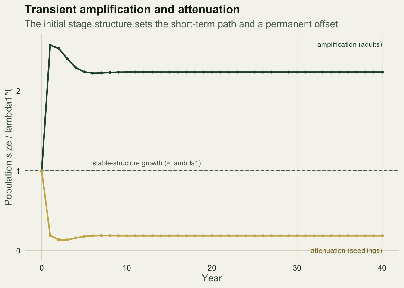
c(large_first_step = ps_large[2], large_peak = max(ps_large), large_inertia = ps_large[Tt + 1],
  seed_first_step = ps_seed[2], seed_trough = min(ps_seed), seed_inertia = ps_seed[Tt + 1])
large_first_step large_peak large_inertia seed_first_step
2.5711104 2.5711104 2.2338058 0.1904526
seed_trough seed_inertia
0.1351404 0.1863117 The two populations share the same matrix and the same asymptotic rate, yet they end up on permanently different tracks. The adult-started population settles at an inertia of about 2.23, meaning it is more than twice as large as it would have been from a stable start; the seedling-started one settles at about 0.19, roughly a fifth. The ratio between the two eventual sizes is about twelve, the same factor as the reproductive-value gap between large adults and seedlings. Asymptotic growth is identical; the head start is not.
How fast the transient fades
The damping ratio predicts the convergence speed. Measuring the distance between the current stage distribution and the stable one, on a log scale, gives a line whose slope is set by the damping ratio: the distance decays geometrically at one over the damping ratio per year.
dist_series <- function(n0) {
  x <- n0; dvec <- numeric(Tt + 1)
  for (t in 0:Tt) {
    nn <- x / sum(x); dvec[t + 1] <- 0.5 * sum(abs(nn - w))
    x <- as.numeric(A %*% x)
  }
  dvec
}
dL <- dist_series(n_large); dS <- dist_series(n_seed)
ref <- dL[3] * (1 / damping)^((0:Tt) - 2); ref[1:3] <- NA

df2 <- bind_rows(
  data.frame(year = 0:Tt, dist = dL, init = "Start: all large adults"),
  data.frame(year = 0:Tt, dist = dS, init = "Start: all seedlings"))
df2 <- df2[df2$dist > 1e-6, ]
refdf <- data.frame(year = 0:Tt, ref = ref)
refdf <- refdf[!is.na(refdf$ref) & refdf$ref > 1e-6, ]

ggplot(df2, aes(year, dist, colour = init)) +
  geom_line(data = refdf, aes(year, ref), inherit.aes = FALSE,
            colour = te_brick, linetype = "22", linewidth = 0.7) +
  geom_line(linewidth = 0.8) + geom_point(size = 1.0) +
  scale_colour_manual(values = c("Start: all large adults" = te_forest,
                                 "Start: all seedlings" = te_gold)) +
  scale_y_log10() +
  annotate("text", x = 22, y = ref[which(!is.na(ref))][18] * 2.4,
           label = "slope = (1 / damping ratio)^t", colour = te_brick, hjust = 0, size = 3.1) +
  labs(title = "Convergence to the stable stage structure",
       subtitle = "Distance to the stable distribution decays geometrically at the damping ratio",
       x = "Year", y = "Distance to stable structure (log scale)") +
  theme_te()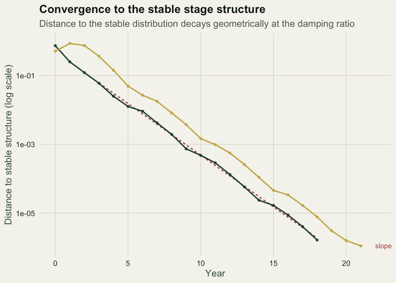
Both curves run parallel to the reference slope on the log scale, confirming that the damping ratio governs the rate of return. The seedling-started curve wobbles as it descends because the subdominant eigenvalue here is complex, so convergence oscillates rather than sliding straight in, but the average rate is the same. A larger damping ratio would pull both curves down faster and shorten the transient; a ratio near one would leave the population lingering far from its stable structure for a long time.
Where to go next
Transient indices sharpen the reading of any matrix model. Where a prospective sensitivity analysis asks how the asymptotic rate would respond to a change in a vital rate, the transient measures ask what happens in the years before the asymptotic rate takes hold, which is exactly the window a reintroduction or a harvest operates in. Stott and colleagues give a full catalogue of these indices and the packages that compute them; the eigenvalues, stable structure and subdominant root used here come straight from the Leslie and Lefkovitch posts, and the amplification bounds tie back to the reproductive values that drive sensitivity.
References
Neubert MG, Caswell H 1997. Ecology 78(3):653-665 (10.1890/0012-9658(1997)078[0653:ATRFMT]2.0.CO;2).
Stott I, Townley S, Hodgson DJ 2011. Ecology Letters 14(9):959-970 (10.1111/j.1461-0248.2011.01659.x).
Koons DN, Grand JB, Zinner B, Rockwell RF 2005. Ecological Modelling 185(2-4):283-297 (10.1016/j.ecolmodel.2004.12.011).
Caswell H 2001. Matrix Population Models: Construction, Analysis, and Interpretation, 2nd edition. Sinauer Associates. ISBN 978-0-87893-096-8.