library(ggplot2)
library(patchwork)

te_paper  <- "#f5f4ee"
te_ink    <- "#16241d"
te_body   <- "#2c3a31"
te_forest <- "#275139"
te_rust   <- "#b5534e"
te_gold   <- "#c9b458"
te_line   <- "#dad9ca"

theme_datasheet <- function() {
  theme_minimal(base_size = 12) +
    theme(plot.background  = element_rect(fill = te_paper, colour = NA),
          panel.background = element_rect(fill = te_paper, colour = NA),
          panel.grid.major = element_line(colour = te_line, linewidth = 0.3),
          panel.grid.minor = element_blank(),
          text             = element_text(colour = te_body),
          plot.title       = element_text(colour = te_ink, face = "bold"),
          plot.subtitle    = element_text(colour = te_body),
          axis.text        = element_text(colour = te_body))
}

fecundity_3 <- 6
surv_juv    <- 0.5

semel <- matrix(0, 3, 3)
semel[1, 3] <- fecundity_3
semel[2, 1] <- surv_juv
semel[3, 2] <- surv_juv

ev_semel  <- eigen(semel)
naive_lam <- Re(ev_semel$values[1])
true_lam  <- max(Mod(ev_semel$values))
mod_all <- Mod(ev_semel$values)Checking a matrix population model
R
population dynamics
demography
matrix models
ecology tutorial
Four checks on a population projection matrix before you read lambda off it: primitivity, reducibility, stage duration, and how wide the interval really is.
A projection matrix is easy to build and easy to read. Fill in survival, fill in fecundity, take the dominant eigenvalue, report it as the annual growth rate. Every step is one line of R, and the output is a single number that people will quote.
The trouble is that three of those lines have failure modes that produce output rather than errors. eigen() will hand back a number for any square matrix, including matrices for which the leading eigenvalue is not the growth rate of anything. A stage matrix built from stated stage durations will project a population that grows at the wrong rate if the durations were converted the obvious way. And a lambda quoted without an interval is usually being asked to support a claim that its own data cannot support.
This post runs four checks over a matrix before its lambda is allowed out. Each one is a few lines of base R, and each one is here because it catches a mistake that survives every other kind of inspection.
Check one: is the matrix primitive?
A Leslie matrix for a semelparous animal with a fixed three year cycle reproduces only at age three. That is a perfectly sensible piece of biology, and it breaks the standard idiom.
The naive reading, the first eigenvalue with its imaginary part discarded, gives -0.572. That is not a growth rate at all: a population multiplied by a negative number would alternate in sign. The correct answer, the eigenvalue of largest modulus, is 1.1447, and the population is growing.
The reason both numbers exist is that all three eigenvalues have the same modulus, 1.1447, so there is no unique leading eigenvalue for eigen() to sort to the top, and the complex pair happens to come first. Equal moduli make the damping ratio exactly one, which is another way of saying the transient never dies.
mat_pow <- function(A, k) {
  B <- diag(nrow(A))
  for (i in seq_len(k)) B <- B %*% A
  B
}
primitive_power <- function(A, k_max = (nrow(A) - 1)^2 + 1) {
  for (k in seq_len(k_max)) if (all(mat_pow(A, k) > 0)) return(k)
  NA_integer_
}

semel_prim <- primitive_power(semel)

n_start  <- 100
n_year   <- 15
project  <- function(A, n0, years) {
  out <- matrix(NA_real_, years + 1, length(n0))
  out[1, ] <- n0
  for (t in seq_len(years)) out[t + 1, ] <- as.numeric(A %*% out[t, ])
  out
}
traj_semel <- project(semel, c(n_start, 0, 0), n_year)
tot_semel  <- rowSums(traj_semel)
step_ratio <- tot_semel[-1] / tot_semel[-length(tot_semel)]
cycle_gain <- prod(step_ratio[1:3])
primitive_power() returns NA: no power of the matrix up to the bound has every entry positive, which is what imprimitive means. A projection confirms what that means in practice. Starting from a hundred newborns, the year on year multiplier repeats 0.50, 0.50, 6.00 forever. It never settles on anything. The product over one cycle is 1.5, and the cube root of that is 1.1447, which is the lambda the eigenvalue was trying to report: a long run average that no single year ever realises.
semel2 <- semel
semel2[1, 2] <- 1.2
traj2   <- project(semel2, c(n_start, 0, 0), n_year)
prim2   <- primitive_power(semel2)
lam2    <- max(Mod(eigen(semel2)$values))
damp2   <- lam2 / sort(Mod(eigen(semel2)$values), decreasing = TRUE)[2]

cyc <- data.frame(year = 0:n_year, total = tot_semel, panel = "breeds at age 3 only")
smo <- data.frame(year = 0:n_year, total = rowSums(traj2), panel = "breeds at ages 2 and 3")
both <- rbind(cyc, smo)
both$panel <- factor(both$panel, levels = c("breeds at age 3 only", "breeds at ages 2 and 3"))

ggplot(both, aes(year, total)) +
  geom_line(colour = te_forest, linewidth = 0.9) +
  geom_point(colour = te_forest, size = 1.8) +
  scale_y_log10() +
  facet_wrap(~panel) +
  labs(x = "year", y = "population total (log scale)",
       title = "One matrix converges, the other never does",
       subtitle = "same survival, same fecundity at age three") +
  theme_datasheet() +
  theme(strip.text = element_text(colour = te_ink, face = "bold"))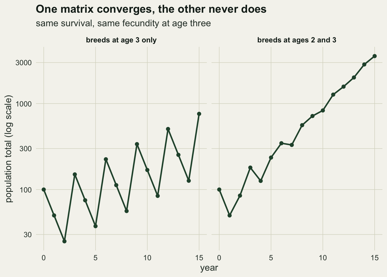
Adding reproduction at age two makes every entry of the 5th power positive, gives a damping ratio of 1.24, and the wobble fades instead of repeating. The biology of the two cases is not very different. The behaviour of the standard summary statistic is completely different.
Use max(Mod(eigen(A)$values)) rather than Re(eigen(A)$values[1]) in every case, and run the primitivity test whenever reproduction is confined to a narrow band of ages. On an imprimitive matrix the eigenvalue is still a long run average, but the stable stage distribution, the damping ratio and every transient measure built on the subdominant eigenvalue stop meaning what their names suggest.
Check two: is the matrix irreducible?
The second failure is quieter, because it returns a real number in the first slot and nothing looks wrong.
stage_names <- c("seedling", "small", "medium", "large")
A_full <- matrix(c(0.00, 0.00, 1.80, 4.50,
                   0.35, 0.42, 0.00, 0.00,
                   0.00, 0.28, 0.55, 0.10,
                   0.00, 0.00, 0.22, 0.86), 4, 4, byrow = TRUE,
                 dimnames = list(stage_names, stage_names))

lambda_of <- function(A) max(Mod(eigen(A)$values))
stable_of <- function(A) {
  e <- eigen(A); i <- which.max(Mod(e$values))
  w <- Re(e$vectors[, i]); w / sum(w)
}

A_slip <- A_full
A_slip["large", "medium"] <- 0     # the transition into the largest stage, lost

lam_full <- lambda_of(A_full)
lam_slip <- lambda_of(A_slip)
w_slip   <- stable_of(A_slip)

is_irreducible <- function(A) {
  n <- nrow(A)
  all(mat_pow((A > 0) + diag(n), n - 1) > 0)
}
irr_full <- is_irreducible(A_full)
irr_slip <- is_irreducible(A_slip)
Deleting one transition, the one that moves medium plants into the largest stage, takes lambda from 1.172 to 0.926. A population growing at 17.2 per cent a year becomes one declining at 7.4 per cent a year, and both numbers are plausible for a plant. Nothing in the output announces that a cell was lost.
The stable stage distribution does announce it. It reads 0.453, 0.313, 0.233, 0.000: the largest stage holds exactly zero of the population, forever, because nothing can get into it. is_irreducible() says TRUE for the intended matrix and FALSE for the damaged one, and it is a one line test on the digraph of nonzero entries.
Read the stable stage vector every time, even when the question is only about lambda. A structural zero in it is either a real dead end in the life cycle or a typing error, and a matrix that has both a plausible lambda and an impossible stage vector will pass any check that looks at lambda alone.
Check three: were stage durations converted properly?
Stage matrices are usually built from a table of stated survivals and stated stage durations: a medium plant survives at some annual rate and takes some number of years to reach the next stage. The obvious conversion is that one over the duration is the fraction of survivors moving on each year. It is wrong, and the error runs the same way every time.
surv <- c(0.42, 0.68, 0.80, 0.91)
dur  <- c(2, 3, 5, 1)
fec  <- c(0, 0, 1.9, 7.4)
n_st <- length(surv)
surv_demo <- 0.55
dur_demo  <- 10

build_stage <- function(gam) {
  A <- matrix(0, n_st, n_st, dimnames = list(stage_names, stage_names))
  A[1, ] <- fec
  for (i in seq_len(n_st - 1)) {
    A[i, i]     <- A[i, i] + surv[i] * (1 - gam[i])
    A[i + 1, i] <- surv[i] * gam[i]
  }
  A[n_st, n_st] <- A[n_st, n_st] + surv[n_st]
  A
}

gamma_fixed <- function(s, d, lam) {
  x <- s / lam
  (x^d - x^(d - 1)) / (x^d - 1)
}

gam_naive <- c(1 / dur[-n_st], 0)
gam_unit  <- c(gamma_fixed(surv[-n_st], dur[-n_st], 1), 0)

lam_iter <- 1
for (it in seq_len(60)) {
  gam_iter <- c(gamma_fixed(surv[-n_st], dur[-n_st], lam_iter), 0)
  lam_iter <- lambda_of(build_stage(gam_iter))
}
Here the medium stage survives at 0.80 a year and takes 5 years to clear, so the obvious conversion advances a fifth of the survivors annually. The correct conversion comes instead from asking what fraction of a stage’s occupants are in their last year of it. In a population growing at lambda, the number of individuals who entered the stage j years ago is proportional to (s / lambda)^j, so the fraction ready to move on is a ratio of a geometric series rather than one over the duration. That expression contains lambda, which is the thing being computed, so it has to be iterated.
There is a ground truth available here, because a stage of fixed duration can be written out exactly, one age class per year within each stage. That expanded matrix needs no approximation at all, and it is what the collapsed four by four version is trying to imitate.
expand_stages <- function() {
  k   <- sum(dur)
  A   <- matrix(0, k, k)
  idx <- split(seq_len(k), rep(seq_along(dur), dur))
  for (i in seq_along(dur)) {
    v <- idx[[i]]
    for (j in seq_along(v)) {
      if (j < length(v))            A[v[j + 1], v[j]]      <- surv[i]
      else if (i < length(dur))     A[idx[[i + 1]][1], v[j]] <- surv[i]
      else                          A[v[j], v[j]]          <- surv[i]
      A[1, v[j]] <- A[1, v[j]] + fec[i]
    }
  }
  list(A = A, idx = idx)
}
xp        <- expand_stages()
lam_exact <- lambda_of(xp$A)
w_exact   <- vapply(xp$idx, function(v) sum(stable_of(xp$A)[v]), 0)

lam_naive <- lambda_of(build_stage(gam_naive))
lam_unit  <- lambda_of(build_stage(gam_unit))
w_iter    <- stable_of(build_stage(gam_iter))
w_naive   <- stable_of(build_stage(gam_naive))

err_naive <- 100 * (lam_naive / lam_exact - 1)
err_unit  <- 100 * (lam_unit  / lam_exact - 1)
err_iter  <- 100 * (lam_iter  / lam_exact - 1)
fold_naive <- (lam_naive - 1) / (lam_exact - 1)
ratio_demo <- (1 / dur_demo) / gamma_fixed(surv_demo, dur_demo, 1)
The exact 11 by 11 matrix gives 1.0374. Dividing one by the duration gives 1.1465, which is +10.5 per cent high: a population growing at 3.7 per cent a year reported as growing at 14.6 per cent, 3.9 times as fast. The fixed duration formula evaluated at lambda equal to one gives 1.0455, an error of +0.78 per cent. Iterating it to convergence gives 1.0374, an error of +0.00 per cent, and the aggregated stable stage distribution then matches the exact one to four decimal places.
sweep_dur <- expand.grid(d = 2:12, s = c(0.55, 0.75, 0.92))
sweep_dur$gam   <- gamma_fixed(sweep_dur$s, sweep_dur$d, 1)
sweep_dur$naive <- 1 / sweep_dur$d
sweep_dur$lab   <- factor(sprintf("s %.2f", sweep_dur$s))

p_gam <- ggplot(sweep_dur, aes(d, gam, colour = lab)) +
  geom_line(aes(y = naive), colour = te_ink, linetype = "dashed", linewidth = 0.7) +
  geom_line(linewidth = 0.9) +
  scale_colour_manual(values = c(te_rust, te_gold, te_forest), name = NULL) +
  scale_x_continuous(breaks = seq(2, 12, 2)) +
  labs(x = "stated stage duration (years)", y = "fraction advancing each year",
       title = "The right fraction is smaller",
       subtitle = "dashed: one over duration") +
  theme_datasheet() + theme(legend.position = "bottom")

bars <- data.frame(
  what = factor(c("exact", "one over T", "fixed", "fixed, iterated"),
                levels = c("exact", "one over T", "fixed", "fixed, iterated")),
  lam  = c(lam_exact, lam_naive, lam_unit, lam_iter))

p_bar <- ggplot(bars, aes(what, lam)) +
  geom_col(fill = te_forest, width = 0.6) +
  geom_hline(yintercept = lam_exact, colour = te_rust, linetype = "dashed",
             linewidth = 0.7) +
  coord_cartesian(ylim = c(0.95, 1.2)) +
  labs(x = NULL, y = "lambda", title = "And it inflates lambda",
       subtitle = "dashed red: the exact answer") +
  theme_datasheet() +
  theme(axis.text.x = element_text(angle = 20, hjust = 1))

p_gam + p_bar + plot_annotation(theme = theme_datasheet())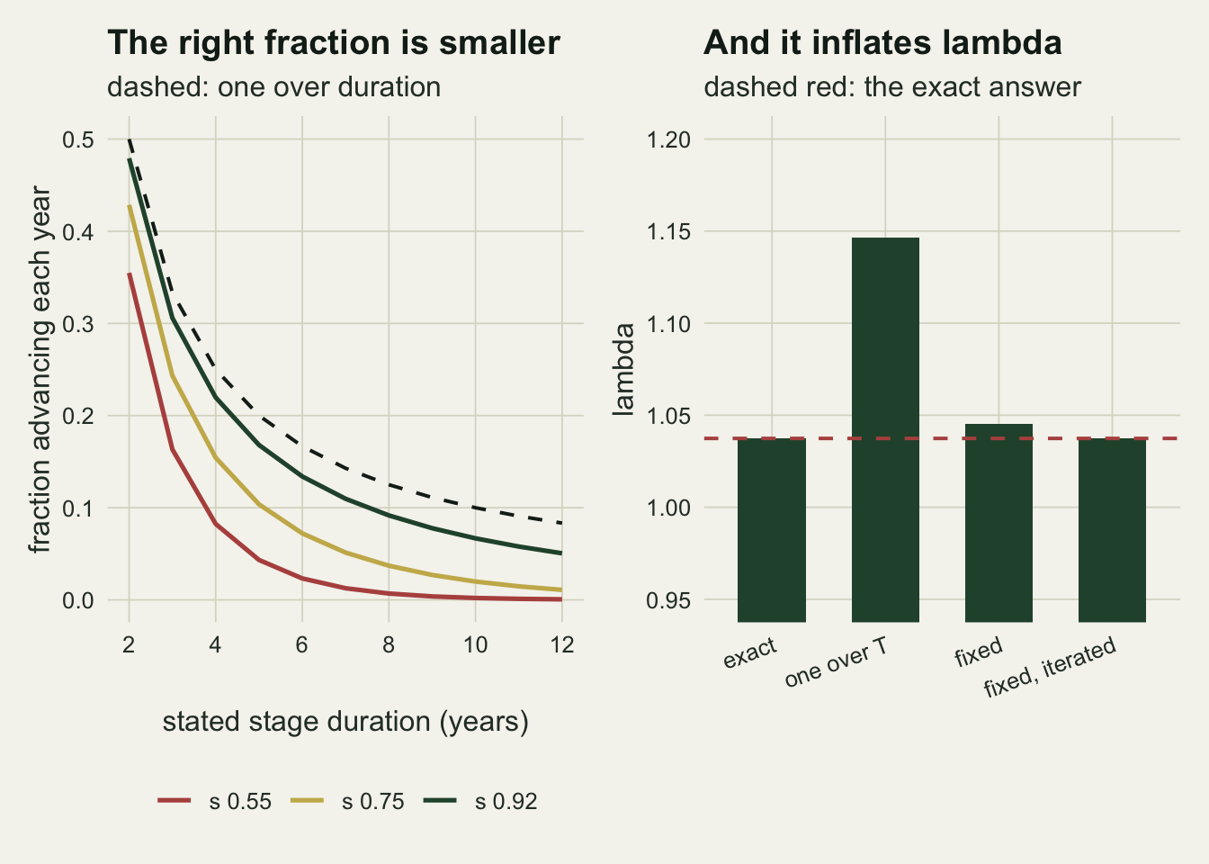
The gap widens with duration and with mortality. At a survival of 0.55 and a duration of 10 years, the naive fraction is 48.1 times the correct one, because with heavy mortality almost nobody is left in the stage long enough to be in its final year.
Both fixed duration versions are close enough that the iteration is a refinement rather than a rescue. The naive version is not a refinement of anything.
Check four: how wide is the interval on lambda?
Every number above is treated as known. In a real study each survival came from a handful of marked individuals and each fecundity from a handful of counted broods, and lambda inherits all of that.
build_stage_from <- function(sv, gm, fc) {
  A <- matrix(0, n_st, n_st)
  A[1, ] <- fc
  for (i in seq_len(n_st - 1)) {
    A[i, i]     <- A[i, i] + sv[i] * (1 - gm[i])
    A[i + 1, i] <- sv[i] * gm[i]
  }
  A[n_st, n_st] <- A[n_st, n_st] + sv[n_st]
  A
}

A_true  <- build_stage(gam_iter)
stay    <- diag(A_true)
advance <- c(A_true[2, 1], A_true[3, 2], A_true[4, 3], 0)

n_mark_base <- c(120, 80, 60, 40)
n_fem_base  <- c(0, 0, 45, 30)
n_boot      <- 2000
effort      <- c(1, 2, 4, 8)

boot_lambda <- function(mult, seed) {
  set.seed(seed)
  n_mark <- n_mark_base * mult
  n_fem  <- n_fem_base  * mult
  vapply(seq_len(n_boot), function(b) {
    sv <- numeric(n_st); gm <- numeric(n_st)
    for (i in seq_len(n_st)) {
      pr  <- if (i == n_st) c(stay[i], 0, 1 - stay[i])
             else c(stay[i], advance[i], 1 - stay[i] - advance[i])
      cnt <- rmultinom(1, n_mark[i], pr)[, 1]
      sv[i] <- (cnt[1] + cnt[2]) / n_mark[i]
      gm[i] <- if (sv[i] > 0) cnt[2] / (cnt[1] + cnt[2]) else 0
    }
    fc <- c(0, 0, mean(rpois(n_fem[3], fec[3])), mean(rpois(n_fem[4], fec[4])))
    lambda_of(build_stage_from(sv, gm, fc))
  }, 0)
}

boot_all <- lapply(seq_along(effort), function(j) boot_lambda(effort[j], 900 + j))
ci <- t(vapply(boot_all, function(v) c(quantile(v, 0.025), quantile(v, 0.975),
                                       mean(v > 1)), numeric(3)))
colnames(ci) <- c("lo", "hi", "p_growing")
ci_tab <- data.frame(marked = sum(n_mark_base) * effort, ci)
ci_pct      <- 97.5
tiny_entry  <- 1e-9
boot_mc_se  <- sd(boot_all[[1]]) / sqrt(n_boot)
At the base level of effort, 300 marked individuals plus 75 fecundity records, the interval on lambda runs from 0.951 to 1.115. The point estimate is 1.037 and the data cannot distinguish it from a stationary population: 80 per cent of the resampled matrices grow, which is a long way from the 97.5 per cent that would be needed to exclude one.
dens <- do.call(rbind, lapply(seq_along(boot_all), function(j)
  data.frame(lambda = boot_all[[j]],
             effort = sprintf("%d marked", sum(n_mark_base) * effort[j]))))
dens$effort <- factor(dens$effort,
                      levels = sprintf("%d marked", sum(n_mark_base) * effort))

ggplot(dens, aes(lambda, colour = effort)) +
  geom_density(linewidth = 0.9) +
  geom_vline(xintercept = 1, colour = te_ink, linetype = "dashed", linewidth = 0.7) +
  geom_vline(xintercept = lam_iter, colour = te_gold, linewidth = 0.7) +
  scale_colour_manual(values = c(te_rust, te_gold, te_forest, te_ink), name = NULL) +
  labs(x = "lambda", y = "density",
       title = "The growth rate a demographic study can actually resolve",
       subtitle = "dashed black: stationary; solid gold: the matrix used to generate the data") +
  theme_datasheet() + theme(legend.position = "bottom")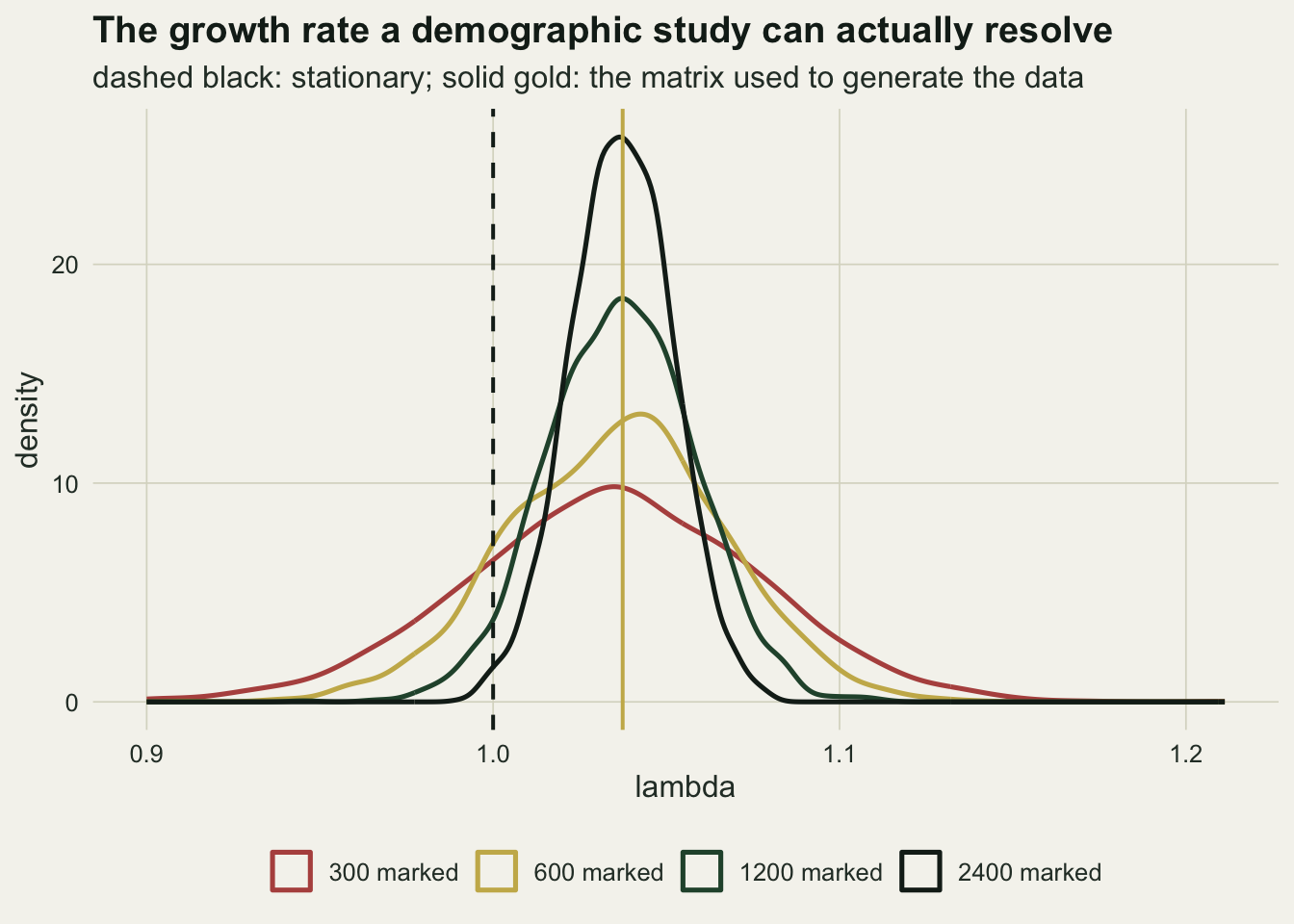
Quadrupling the effort to 1200 marked individuals narrows the interval to 0.995 to 1.078, which still contains one. Only at 2400 marked individuals does the interval clear it, running from 1.008 to 1.065 with 99 per cent of resampled matrices growing. A 4 per cent annual growth rate is a real quantity, and separating it from zero takes a study several times the size of the one most people run.
What to check, in order
Compute lambda as max(Mod(eigen(A)$values)). It costs nothing, it is right when the naive version is right, and it does not silently return a complex root’s real part when reproduction is confined to one age.
Test primitivity and irreducibility before reading any eigenvector. Two short functions on matrix powers cover both, and between them they catch narrow breeding windows, absorbing stages and transitions lost in transcription.
Print the stable stage distribution alongside lambda. A zero or a near zero in it is the cheapest available detector of a structural mistake, and it is visible even when lambda looks entirely reasonable.
Convert stage durations with the fixed duration expression rather than one over the duration, and iterate it. If the stages are few and the durations short, write the expanded age within stage matrix instead and skip the approximation.
Put an interval on lambda. A parametric bootstrap from the counts that produced each rate is twenty lines, and it will frequently show that the sign of the growth rate is not established.
Honest limits
The bootstrap here assumes the sampling design it simulates: independent individuals, survival and transition observed without error, fecundity counted without error, and no year to year variation in the vital rates. Real studies violate all four. Detection error alone inflates the interval further, and environmental variation changes the question from what lambda is to what the stochastic growth rate is, which is a different quantity with different arithmetic.
The fixed duration conversion assumes exactly what its name says: every individual spends the same number of years in the stage. When duration itself varies among individuals, no single advancement fraction reproduces the age structure, and the collapsed matrix is an approximation whose error is not bounded by anything shown here. The expanded matrix is exact only for the fixed duration case as well.
The primitivity and irreducibility tests are structural: they look at which entries are nonzero, not at how big they are. A matrix with a transition of 1e-09 passes both tests and behaves in every practical sense like one that fails them. Convergence in that case is arbitrarily slow rather than absent, which is a distinction the mathematics cares about more than a field ecologist does.
The four checks are structural and statistical, and none of them asks whether the stages are the right stages. A matrix that passes every test here can still be built on a classification that splits the life cycle in a place where the vital rates do not change, or lumps two groups whose survival differs by a factor of two. That is the largest source of error in the whole exercise and the one no diagnostic reaches.
Finally, the bootstrap uses 2000 resamples, which puts a Monte Carlo error of roughly 0.0009 on each interval endpoint at the base effort level. The endpoints are quoted to three decimals for tidiness; the third decimal is not stable.
References
Stott I, Townley S, Carslake D, Hodgson DJ 2010 Methods in Ecology and Evolution 1(3):242-252 (10.1111/j.2041-210X.2010.00032.x)
Kendall BE, Fujiwara M, Diaz-Lopez J, Schneider S, Voigt J, Wiesner S 2019 Ecological Modelling 406:33-43 (10.1016/j.ecolmodel.2019.03.011)
Crouse DT, Crowder LB, Caswell H 1987 Ecology 68(5):1412-1423 (10.2307/1939225)