Life table response experiments (LTRE) in R

Decompose the difference in growth between two matrices into per-element contributions in R, and see why the biggest vital-rate change need not matter most.

Sensitivity analysis is prospective: it asks how the growth rate would respond to a hypothetical change in a vital rate. A life table response experiment turns the question around. Two populations, say a control and a treatment, or two sites, or two years, actually differ in their vital rates, and their growth rates differ as a result. The LTRE decomposes that observed difference in growth into a sum of contributions, one per matrix element, so you can see which rate differences drove the outcome. The headline lesson, which Caswell set out in 1989, is that a large difference in a vital rate need not produce a large contribution, because contribution is the difference weighted by how sensitive growth is to that rate. This post builds the decomposition in base R and shows exactly that reversal.

Two matrices to compare

The example is a long-lived plant measured under a control and a treatment. The treatment raises fecundity sharply but carries a survival cost, a classic reproduction trade-off, and also improves two growth transitions a little.

library(ggplot2)
library(dplyr)
library(tidyr)

A_control <- matrix(c(0,    0,    1.0,
                      0.30, 0.30, 0,
                      0,    0.26, 0.90), nrow = 3, byrow = TRUE)
A_treat   <- matrix(c(0,    0,    1.8,
                      0.34, 0.30, 0,
                      0,    0.30, 0.80), nrow = 3, byrow = TRUE)

lambda <- function(A) {
  ev <- eigen(A); Re(ev$values[which.max(Re(ev$values))])
}
lam_c <- lambda(A_control); lam_t <- lambda(A_treat)
c(lambda_control = lam_c, lambda_treatment = lam_t, delta_lambda = lam_t - lam_c)

  lambda_control lambda_treatment     delta_lambda 
       1.0090260        1.0390761        0.0300501 

The control grows at almost exactly replacement, about 1.009, and the treatment a little faster, about 1.039, a difference in growth of about 0.030. On its own that tells you the treatment helped slightly. It does not tell you why, given that the treatment nearly doubled fecundity yet also cut adult survival.

Sensitivities at the midpoint

The decomposition weights each vital-rate difference by the sensitivity of growth to that element. Caswell’s recommendation is to evaluate the sensitivities at the mean of the two matrices, which keeps the approximation symmetric and accurate. The sensitivity of the dominant eigenvalue to element (i, j) is the reproductive value of stage i times the abundance of stage j, divided by their weighted product.

sensitivity <- function(A) {
  ev <- eigen(A); i <- which.max(Re(ev$values))
  w <- Re(ev$vectors[, i])
  evL <- eigen(t(A)); iL <- which.max(Re(evL$values))
  v <- Re(evL$vectors[, iL])
  outer(v, w) / sum(v * w)
}
A_mid <- (A_control + A_treat) / 2
S_mid <- sensitivity(A_mid)
round(S_mid, 3)

      [,1]  [,2]  [,3]
[1,] 0.119 0.053 0.087
[2,] 0.380 0.169 0.277
[3,] 0.977 0.434 0.712

The sensitivity matrix shows the familiar pattern for a long-lived species: growth is far more sensitive to adult survival, the bottom-right element, than to fecundity, the top-right one. That gap is what will overturn the raw ranking.

The contributions

Each contribution is the difference in a matrix element multiplied by its midpoint sensitivity. Summed over all elements, the contributions recover the difference in growth.

dA <- A_treat - A_control
contr <- dA * S_mid

cells <- list(c(1, 3), c(3, 3), c(2, 1), c(3, 2))
labels <- c("Fecundity (large adult)", "Adult survival (large stasis)",
            "Growth small to medium", "Growth medium to large")
tab <- data.frame(
  element = labels,
  raw_difference = sapply(cells, function(k) dA[k[1], k[2]]),
  sensitivity = sapply(cells, function(k) round(S_mid[k[1], k[2]], 3)),
  contribution = sapply(cells, function(k) round(contr[k[1], k[2]], 4)))
tab

                        element raw_difference sensitivity contribution
1       Fecundity (large adult)           0.80       0.087       0.0694
2 Adult survival (large stasis)          -0.10       0.712      -0.0712
3        Growth small to medium           0.04       0.380       0.0152
4        Growth medium to large           0.04       0.434       0.0174

c(sum_of_contributions = sum(contr), delta_lambda = lam_t - lam_c,
  residual = (lam_t - lam_c) - sum(contr))

sum_of_contributions         delta_lambda             residual 
        0.0307441647         0.0300500989        -0.0006940658 

The contributions sum to about 0.031, against a true difference in growth of about 0.030. The residual, under one thousandth, is the second-order curvature the linear decomposition drops; for differences this size it is negligible. That closeness is the check that the decomposition is trustworthy.

Now read the table. Fecundity has by far the largest raw difference, a rise of 0.8 that nearly doubles it, but its contribution is only about +0.069 because growth is barely sensitive to fecundity. Adult survival falls by only 0.1, an eighth of the fecundity change, yet its contribution is about minus 0.071, the largest in magnitude of the four, because growth is about eight times more sensitive to it. The biggest raw change is not the biggest contribution.

res <- data.frame(short = c("Fecundity", "Adult survival", "Growth S->M", "Growth M->L"),
                  contr = sapply(cells, function(k) contr[k[1], k[2]]),
                  raw = sapply(cells, function(k) dA[k[1], k[2]]))
res$sign <- ifelse(res$contr >= 0, "pos", "neg")
res1 <- res |> arrange(contr) |> mutate(short = factor(short, levels = short))

ggplot(res1, aes(contr, short, fill = sign)) +
  geom_col(width = 0.62) +
  geom_vline(xintercept = 0, colour = te_faint, linewidth = 0.4) +
  scale_fill_manual(values = c(pos = te_forest, neg = te_brick)) +
  geom_text(aes(label = sprintf("%+.3f", contr),
                hjust = ifelse(contr >= 0, -0.15, 1.15)),
            colour = te_body, size = 3.1) +
  labs(title = "Which vital-rate differences drive the change in growth",
       subtitle = sprintf("Contributions sum to a growth difference of %+.3f", lam_t - lam_c),
       x = "Contribution to the change in growth", y = NULL) +
  coord_cartesian(xlim = c(-0.095, 0.095)) +
  theme_te()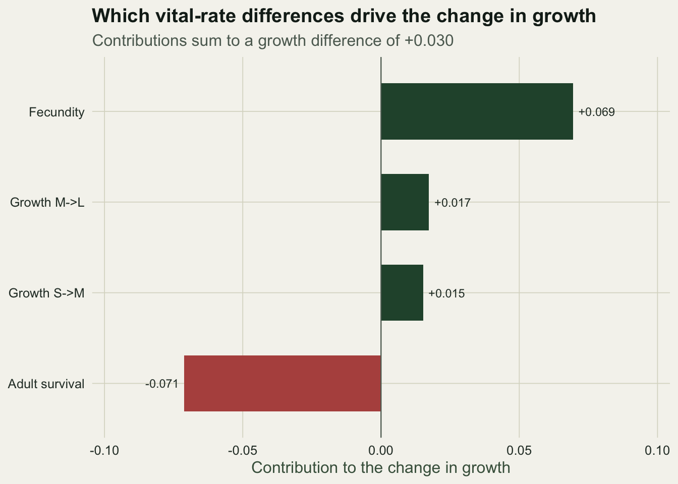

Figure 1: Contribution of each vital-rate difference to the change in growth; positive contributions raise it, negative lower it, and they sum to the total.

The trade-off is now legible. The fecundity gain of about +0.069 and the survival cost of about minus 0.071 nearly cancel, so almost none of the net improvement comes from the dramatic reproductive boost. What tips the balance positive is the pair of modest growth-transition gains, together worth about +0.033. A summary that reported only the fecundity increase would have the biology backwards.

Raw change against contribution

Placing the raw differences and the contributions side by side makes the reordering explicit. Fecundity dominates the left panel and adult survival the right.

ord <- res |> arrange(desc(abs(raw))) |> pull(short)
long <- res |>
  transmute(short,
            `Raw vital-rate difference` = raw,
            `LTRE contribution` = contr) |>
  pivot_longer(-short, names_to = "panel", values_to = "value") |>
  mutate(short = factor(short, levels = rev(ord)),
         panel = factor(panel, levels = c("Raw vital-rate difference", "LTRE contribution")),
         sign = ifelse(value >= 0, "pos", "neg"))

ggplot(long, aes(value, short, fill = sign)) +
  geom_col(width = 0.62) +
  geom_vline(xintercept = 0, colour = te_faint, linewidth = 0.4) +
  scale_fill_manual(values = c(pos = te_forest, neg = te_brick)) +
  facet_wrap(~panel, scales = "free_x") +
  labs(title = "Biggest raw change is not the biggest contribution",
       subtitle = "Fecundity has the largest raw change; adult survival, far more sensitive, contributes most",
       x = NULL, y = NULL) +
  theme_te()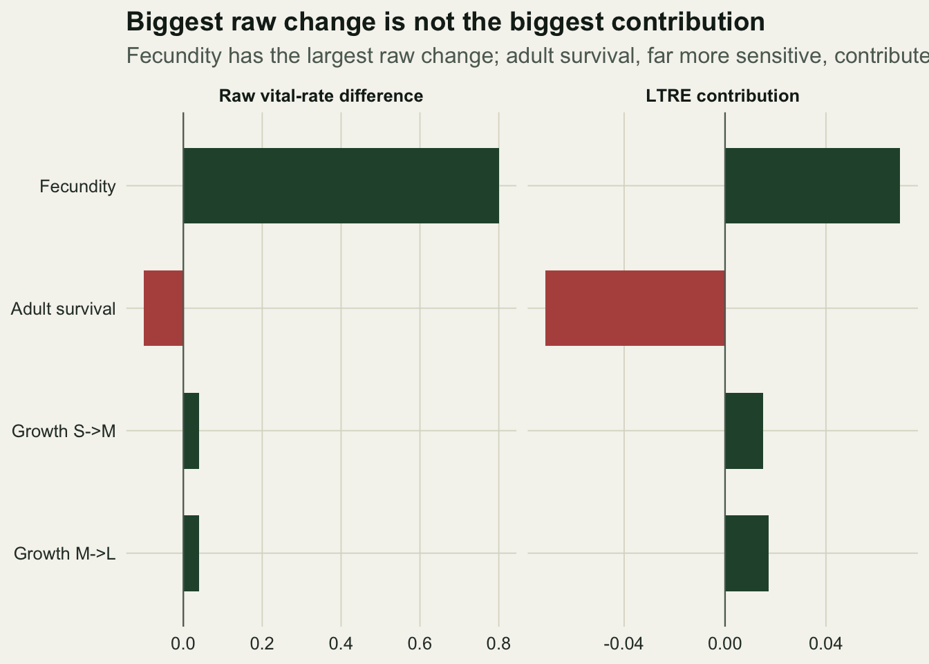

Figure 2: Raw vital-rate differences (left) and their LTRE contributions (right); the largest raw change, fecundity, is not the largest contribution.

Prospective and retrospective, side by side

The two analyses answer different questions and should not be confused. A sensitivity or elasticity analysis is prospective: it takes one matrix and asks which rate to target to raise growth in future, regardless of how much that rate actually varies. An LTRE is retrospective: it takes two matrices that already differ and asks which of the differences that happened accounts for the gap in growth. A rate can be highly sensitive yet contribute nothing to an LTRE because it did not differ between the groups, and a rate can differ a lot yet contribute little because growth is insensitive to it. Reading the two together, the prospective sensitivity from the companion post and the retrospective contribution here, is how you tell what could matter from what did.

References

Caswell H 1989. Ecological Modelling 46(3-4):221-237 (10.1016/0304-3800(89)90019-7).

Caswell H 1996. Ecological Modelling 88(1-3):73-82 (10.1016/0304-3800(95)00070-4).

Caswell H 2000. Ecology 81(3):619-627 (10.1890/0012-9658(2000)081[0619:PARPAT]2.0.CO;2).

de Kroon H, Plaisier A, van Groenendael J, Caswell H 1986. Ecology 67(5):1427-1431 (10.2307/1938700).

Related tutorials

• Matrix sensitivity and elasticity analysis
• Leslie matrix population models in R
• Stage-structured Lefkovitch matrix models
• Stochastic population growth in variable environments