Stochastic population growth in variable environments

How environmental variation lowers the long-run growth of a structured population in R: stochastic lambda by simulation and the Tuljapurkar approximation.

A projection matrix with fixed entries grows at a single asymptotic rate, the dominant eigenvalue lambda. Real vital rates are not fixed: survival, growth and fecundity swing from year to year with weather and resources. Once the matrix itself becomes a random variable, the long-run growth of the population is no longer the dominant eigenvalue of any single matrix, and it is not the average of the annual eigenvalues either. This post builds the stochastic growth rate from scratch in base R, shows why environmental variance is a cost rather than a wash, and checks the classic small-noise approximation against a long simulation.

Two environments, one population

The cleanest model has a small number of environmental states, each with its own matrix. Here a three-stage plant (seedling, juvenile, adult) lives through good years and bad years, drawn independently with fixed probabilities. Good years grow the population, bad years shrink it.

library(ggplot2)
library(dplyr)
library(tidyr)

A_good <- matrix(c(0, 0, 5.6,
                   0.55, 0.25, 0,
                   0, 0.42, 0.90), nrow = 3, byrow = TRUE)
A_bad <- matrix(c(0, 0, 1.4,
                  0.28, 0.18, 0,
                  0, 0.22, 0.78), nrow = 3, byrow = TRUE)

lambda <- function(A) {
  ev <- eigen(A)
  Re(ev$values[which.max(Re(ev$values))])
}

p <- 0.5                      # probability of a good year
Abar <- p * A_good + (1 - p) * A_bad    # the arithmetic mean matrix

c(good = lambda(A_good), bad = lambda(A_bad), mean_matrix = lambda(Abar))

       good         bad mean_matrix 
  1.5458083   0.9098644   1.2194600 

Good years have a growth rate of about 1.55 and bad years about 0.91. The arithmetic mean matrix, formed by averaging the entries with the year frequencies, has a dominant eigenvalue of about 1.22. A naive reading says the population grows at roughly 22 percent per year. It does not.

Simulating the stochastic growth rate

The honest answer comes from running the sequence of matrices forward. Each year draws a matrix, multiplies the current stage vector, and records the log of the one-step total growth. To avoid numerical overflow the vector is renormalised to sum to one after every step, which does not change the growth increments. The stochastic growth rate is the long-run mean of those log increments, written log lambda_s.

sim_loglambda <- function(A_good, A_bad, p, steps, burnin, seed) {
  set.seed(seed)
  n <- rep(1/3, 3)
  lg <- numeric(steps)
  for (t in seq_len(steps)) {
    A <- if (runif(1) < p) A_good else A_bad
    n1 <- as.numeric(A %*% n)
    total <- sum(n1)
    lg[t] <- log(total)
    n <- n1 / total
  }
  mean(lg[(burnin + 1):steps])
}

loglam_s <- sim_loglambda(A_good, A_bad, p, steps = 50000, burnin = 1000, seed = 4242)
c(log_lambda_s = loglam_s, lambda_s = exp(loglam_s),
  log_lambda_meanmatrix = log(lambda(Abar)))

         log_lambda_s              lambda_s log_lambda_meanmatrix 
            0.1626244             1.1765947             0.1984081 

The stochastic growth rate is about 0.163 on the log scale, or a multiplicative rate of about 1.177. That sits well below the mean-matrix value of 1.219. Averaging good and bad years as matrices, then taking an eigenvalue, overstates the real long-run growth. Averaging the two eigenvalues is worse still: the arithmetic mean of 1.55 and 0.91 is about 1.23, further from the truth. The long run is governed by something closer to a geometric mean.

lam_g <- lambda(A_good); lam_b <- lambda(A_bad)
c(arithmetic_mean_lambda = p * lam_g + (1 - p) * lam_b,
  geometric_mean_lambda  = exp(p * log(lam_g) + (1 - p) * log(lam_b)),
  stochastic_lambda_s    = exp(loglam_s))

arithmetic_mean_lambda  geometric_mean_lambda    stochastic_lambda_s 
              1.227836               1.185949               1.176595 

The geometric mean of the two rates, about 1.19, is close to the simulated stochastic rate but not exactly equal to it, because the population never sits at either environment’s stable structure for long. The simulation is the reference value. The intuition, though, is old: multiplicative growth punishes variance, so a bad year costs more than a good year of the same size gains back. Lewontin and Cohen made the point in 1969: a population can have an expected size that grows without bound while its probability of extinction still approaches one, precisely because the geometric and arithmetic mean rates differ.

loglam_bar <- log(lambda(Abar))
ev <- eigen(Abar)
w <- Re(ev$vectors[, which.max(Re(ev$values))]); w <- w / sum(w)

set.seed(919)
years <- 30; nrep <- 6
traj <- lapply(seq_len(nrep), function(r) {
  n <- w * 100; tot <- numeric(years + 1); tot[1] <- sum(n)
  for (t in seq_len(years)) {
    A <- if (runif(1) < p) A_good else A_bad
    n <- as.numeric(A %*% n); tot[t + 1] <- sum(n)
  }
  data.frame(year = 0:years, N = tot, rep = factor(r))
}) |> bind_rows()

det <- data.frame(year = 0:years, N = 100 * exp(loglam_bar * (0:years)))
sto <- data.frame(year = 0:years, N = 100 * exp(loglam_s * (0:years)))

ggplot(traj, aes(year, N, group = rep)) +
  geom_line(colour = te_sage, linewidth = 0.5, alpha = 0.9) +
  geom_line(data = det, aes(year, N), inherit.aes = FALSE,
            colour = te_brick, linewidth = 1.0, linetype = "22") +
  geom_line(data = sto, aes(year, N), inherit.aes = FALSE,
            colour = te_forest, linewidth = 1.0) +
  scale_y_log10() +
  annotate("text", x = years * 0.62, y = det$N[years + 1] * 1.6,
           label = "mean-matrix slope (log lambda-bar)", colour = te_brick, hjust = 0, size = 3.1) +
  annotate("text", x = years * 0.5, y = sto$N[years + 1] * 0.42,
           label = "stochastic slope (log lambda_s)", colour = te_forest, hjust = 0, size = 3.1) +
  labs(title = "Environmental variance lowers long-run growth",
       subtitle = "Six stochastic runs scatter around the stochastic rate, below the mean-matrix rate",
       x = "Year", y = "Total population (log scale)") +
  theme_te()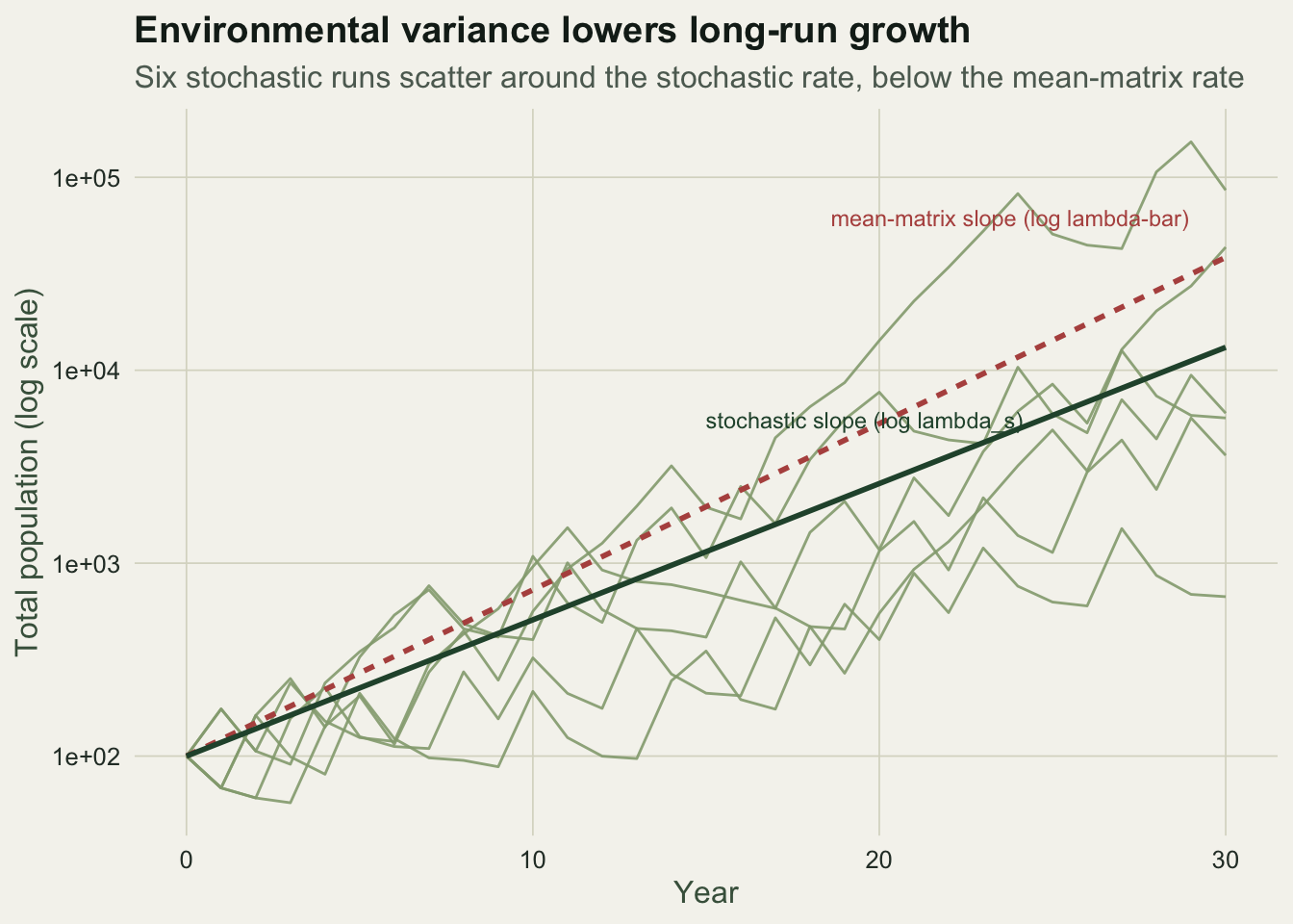

Figure 1: Six stochastic runs (sage) scatter around the stochastic growth rate (forest), below the mean-matrix rate (dashed red).

The Tuljapurkar approximation

Simulating is exact but opaque. Tuljapurkar’s 1982 small-noise approximation gives an analytical formula that separates the two ingredients: the growth you would get from the mean matrix, and the penalty from environmental variance. To first order,

log lambda_s is approximately log(lambda-bar) minus one half of tau-squared divided by lambda-bar squared,

where lambda-bar is the dominant eigenvalue of the mean matrix and tau-squared is the variance in growth that the environment injects, computed through the sensitivities of the mean matrix. When all the variation is driven by a single good-or-bad switch, every matrix entry co-varies perfectly, and the variance term collapses to a compact expression: tau-squared equals p times one-minus-p times the squared sum of the sensitivity-weighted entry differences.

# sensitivities of the mean matrix: S_ij = v_i w_j / (v . w)
w_bar <- Re(ev$vectors[, which.max(Re(ev$values))]); w_bar <- w_bar / sum(w_bar)
evL <- eigen(t(Abar))
v_bar <- Re(evL$vectors[, which.max(Re(evL$values))]); v_bar <- v_bar / v_bar[1]
S <- outer(v_bar, w_bar) / sum(v_bar * w_bar)

dA <- A_good - A_bad
tau2 <- p * (1 - p) * (sum(S * dA))^2
lam_bar <- lambda(Abar)
approx <- log(lam_bar) - 0.5 * tau2 / lam_bar^2

c(sum_S_times_dA = sum(S * dA), tau_squared = tau2,
  approx_log_lambda_s = approx, simulated_log_lambda_s = loglam_s,
  error = approx - loglam_s)

        sum_S_times_dA            tau_squared    approx_log_lambda_s 
           0.642907765            0.103332599            0.163664704 
simulated_log_lambda_s                  error 
           0.162624385            0.001040319 

The approximation lands within about one thousandth of the simulated value. The penalty term is not a rounding detail: without it, the formula returns the mean-matrix rate, which we already know is too high. The variance term drags the prediction down to the simulated stochastic rate. Because it runs through the sensitivities, the formula also tells you which vital rates make variance expensive: an entry that fluctuates a lot but has low sensitivity contributes little, while a modest swing in a high-sensitivity entry can dominate the cost.

Convergence of the estimate

One practical worry with simulation is how long to run it. The running mean of the log increments settles onto the stochastic rate, and its limit is the Tuljapurkar value, comfortably below the mean-matrix line.

set.seed(4242)
Tr <- 3000; n <- rep(1/3, 3); lg <- numeric(Tr)
for (t in seq_len(Tr)) {
  A <- if (runif(1) < p) A_good else A_bad
  n1 <- as.numeric(A %*% n); g <- sum(n1); lg[t] <- log(g); n <- n1 / g
}
runmean <- cumsum(lg) / seq_along(lg)

data.frame(year = seq_len(Tr), rm = runmean) |>
  ggplot(aes(year, rm)) +
  geom_hline(yintercept = loglam_bar, colour = te_brick, linetype = "22", linewidth = 0.7) +
  geom_hline(yintercept = approx, colour = te_gold, linetype = "42", linewidth = 0.7) +
  geom_line(colour = te_forest, linewidth = 0.5) +
  scale_x_log10() +
  annotate("text", x = 3, y = loglam_bar + 0.006,
           label = "log lambda-bar (mean matrix)", colour = te_brick, hjust = 0, size = 3.1) +
  annotate("text", x = 3, y = approx - 0.007,
           label = "Tuljapurkar approximation", colour = te_gold, hjust = 0, size = 3.1) +
  labs(title = "Running estimate of the stochastic growth rate",
       subtitle = "The cumulative mean of log annual growth settles below the mean-matrix value",
       x = "Years simulated (log scale)", y = "Running estimate of log lambda_s") +
  theme_te()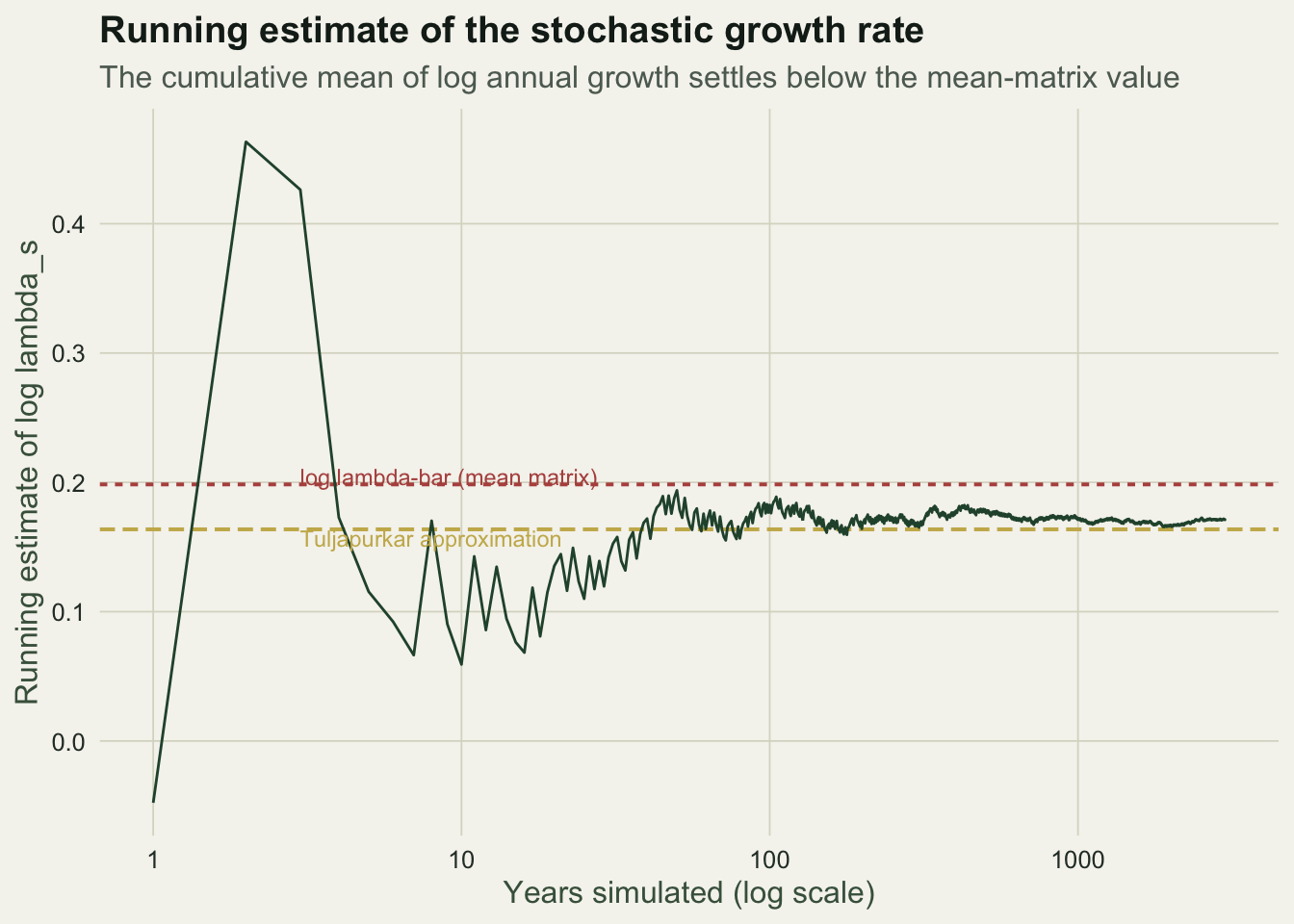

Figure 2: The cumulative mean of log annual growth settles onto the Tuljapurkar value (gold), below the mean-matrix value (dashed red).

Where to go next

The stochastic growth rate is the summary that feeds most quantitative conservation. Its two ingredients, the mean log growth and its variance, are exactly what a count-based population viability analysis estimates from a time series, which is the subject of a companion post. The small-noise approximation also degrades in a predictable way: it assumes the environmental swings are small relative to the mean rates, so with large variance or strong temporal autocorrelation the simulation and the formula part company, and the simulation wins. Autocorrelated environments are handled in the later chapters of Tuljapurkar’s monograph; the deterministic baseline that variance erodes is the ordinary dominant eigenvalue covered in the Leslie and Lefkovitch posts.

References

Lewontin RC, Cohen D 1969. Proceedings of the National Academy of Sciences 62(4):1056-1060 (10.1073/pnas.62.4.1056).

Tuljapurkar SD 1982. Theoretical Population Biology 21(1):114-140 (10.1016/0040-5809(82)90009-0).

Tuljapurkar SD 1990. Population Dynamics in Variable Environments. Lecture Notes in Biomathematics 85, Springer (10.1007/978-3-642-51652-8).

Caswell H 2001. Matrix Population Models: Construction, Analysis, and Interpretation, 2nd edition. Sinauer Associates. ISBN 978-0-87893-096-8.

Related tutorials

• Leslie matrix population models in R
• Stage-structured Lefkovitch matrix models
• Life tables and the population growth rate
• Population viability analysis and extinction risk