Demographic and environmental variance in an IPM

Separating demographic from environmental variance in population growth with an integrated model, why it depends on abundance, and when it is identifiable.

A population’s numbers wobble from year to year for two quite different reasons. One is chance in a finite population: even with fixed vital rates, the number of survivors is a binomial draw and the number of recruits a Poisson draw, so the realised growth rate scatters around its expectation. This demographic noise shrinks as the population grows, because averages over more individuals are steadier. The other reason is the environment: good years and bad years shift survival and recruitment themselves, and this variation does not fade with population size. The two have opposite relationships with abundance, and telling them apart matters for any projection or extinction risk.

Counts alone cannot make the split, because the size of the demographic component depends on the vital rates, which the counts do not identify. An integrated population model (IPM) solves this. The capture-recapture and productivity data pin survival and recruitment, so the demographic variance is known; whatever fluctuation in the counts remains, beyond that known demographic scatter, is environmental. This post fits a state-space count model whose process variance carries both terms and recovers the environmental variance separately, then shows why abundance decides which term dominates and when the environmental part can be estimated at all.

Two kinds of noise, two scalings

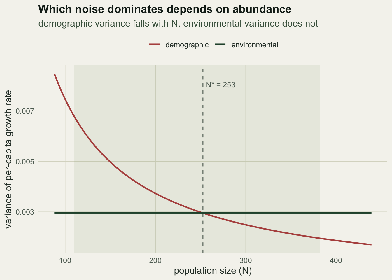
Write the realised per-capita growth rate as its expectation plus scatter. The demographic contribution to its variance is the binomial-plus-Poisson variance divided by population size: survival adds phi(1 - phi) and recruitment adds f, so the demographic variance of the growth rate is phi(1 - phi) + f over N. The environmental contribution is the variance of the rates themselves across years, call it sigma_e squared, and it does not depend on N. Setting the two equal gives a crossover abundance, N* equal to phi(1 - phi) + f divided by sigma_e squared: below it the population is ruled by demographic chance, above it by the environment.

set.seed(133)
Tyr <- 30; phi_bar <- 0.52; f_bar <- 0.48; sig_e <- 0.06; sy_true <- 8; N1_true <- 110

# environmental shocks perturb the rates each year; demographic draws on top
N <- numeric(Tyr); N[1] <- N1_true
for (t in 1:(Tyr - 1)) {
  e    <- rnorm(1, 0, sig_e)
  phit <- plogis(qlogis(phi_bar) + e / (phi_bar + f_bar) * 2)
  ft   <- f_bar * exp(e / (phi_bar + f_bar))
  N[t + 1] <- rbinom(1, N[t], phit) + rpois(1, ft * N[t])
}
C <- round(rnorm(Tyr, N, sy_true))

# capture-recapture and productivity: pin the mean rates (hence demographic size)
p_true <- 0.55; Kcr <- 10; Rrel <- rep(35, Kcr - 1)
recaps <- vector("list", Kcr - 1); never <- integer(Kcr - 1)
for (i in 1:(Kcr - 1)) {
  alive <- rep(TRUE, Rrel[i]); fr <- integer(Rrel[i]); rc <- numeric(Kcr)
  for (t in (i + 1):Kcr) {
    alive <- alive & (runif(length(alive)) < phi_bar)
    got   <- alive & (runif(length(alive)) < p_true) & (fr == 0); fr[got] <- t
  }
  for (t in (i + 1):Kcr) rc[t] <- sum(fr == t)
  recaps[[i]] <- rc; never[i] <- Rrel[i] - sum(fr > 0)
}
Jyr <- 12; prodB <- rep(45, Jyr); prodJ <- rpois(Jyr, prodB * f_bar)

The population runs from 110 to 280 over the 30 years, so its abundance spans a range wide enough to see both regimes.

A process variance with two terms

The count model is a Kalman filter, as in the earlier posts, but the one-step process variance now carries both parts: N times the demographic factor phi(1 - phi) + f, plus N squared times the environmental variance sigma_e squared. The demographic factor is fixed by the survival and recruitment that the capture-recapture and productivity data estimate, so the only new quantity is sigma_e.

marray_ll <- function(phi, p) {
  ll <- 0
  for (i in 1:(Kcr - 1)) {
    ts <- (i + 1):Kcr; q <- phi^(ts - i) * (1 - p)^(ts - i - 1) * p
    ll <- ll + sum(recaps[[i]][ts] * log(q)) + never[i] * log(1 - sum(q))
  }
  ll
}
kf <- function(phi, f, se2, sy, N1, demog = TRUE) {
  lam <- phi + f; dv <- phi * (1 - phi) + f; a <- N1; P <- (2 * sy)^2; ll <- 0
  for (t in seq_along(C)) {
    if (t > 1) {
      ap <- a; a <- lam * ap
      Q  <- (if (demog) dv * max(ap, 1) else 0) + se2 * max(ap, 1)^2
      P  <- lam^2 * P + Q
    }
    F <- P + sy^2; ll <- ll + dnorm(C[t], a, sqrt(F), log = TRUE)
    K <- P / F; a <- a + K * (C[t] - a); P <- (1 - K) * P
  }
  ll
}
nll <- function(par, demog = TRUE) {
  -(kf(plogis(par[1]), exp(par[2]), exp(par[3]), exp(par[4]), exp(par[6]), demog) +
    marray_ll(plogis(par[1]), plogis(par[5])) +
    sum(dpois(prodJ, prodB * exp(par[2]), log = TRUE)))
}
st <- c(qlogis(.5), log(.5), log(0.003), log(9), qlogis(.5), log(C[1]))
of <- optim(st, nll, demog = TRUE, method = "BFGS", hessian = TRUE,
            control = list(maxit = 2000, reltol = 1e-11))
Vf    <- solve(of$hessian)
phi_h <- plogis(of$par[1]); f_h <- exp(of$par[2]); se2_h <- exp(of$par[3])
sig_e_h <- sqrt(se2_h)
ci_lo <- sqrt(exp(of$par[3] - 1.96 * sqrt(Vf[3, 3])))
ci_hi <- sqrt(exp(of$par[3] + 1.96 * sqrt(Vf[3, 3])))
dv_h  <- phi_h * (1 - phi_h) + f_h
Nstar <- dv_h / se2_h

The model recovers the mean rates (survival 0.531, recruitment 0.497) and estimates the environmental standard deviation of the growth rate at 0.054, against a true 0.06. The confidence interval, 0.033 to 0.091, is wide: a thirty-year series holds only so much information about how variable the good and bad years are. The crossover abundance implied by the fit is 253, which sits inside the observed range, so the population passes from demographic to environmental control as it grows.

Ng <- seq(min(N) * 0.8, max(N) * 1.15, length.out = 200)
comp <- rbind(
  data.frame(N = Ng, v = dv_h / Ng, part = "demographic"),
  data.frame(N = Ng, v = se2_h,     part = "environmental")
)
ggplot(comp, aes(N, v, colour = part)) +
  annotate("rect", xmin = min(N), xmax = max(N), ymin = -Inf, ymax = Inf,
           fill = sage, alpha = 0.13) +
  geom_vline(xintercept = Nstar, linetype = "dashed", colour = faint) +
  geom_line(linewidth = 0.9) +
  annotate("text", x = Nstar, y = max(comp$v) * 0.95,
           label = paste0("N* = ", round(Nstar)), colour = faint, hjust = -0.1, size = 3.4) +
  scale_colour_manual(values = c(demographic = rust, environmental = forest), name = NULL) +
  labs(x = "population size (N)", y = "variance of per-capita growth rate",
       title = "Which noise dominates depends on abundance",
       subtitle = "demographic variance falls with N, environmental variance does not") +
  theme_te() + theme(legend.position = "top")

Figure 1: The two contributions to growth-rate variance against population size. The demographic term (rust) falls as one over abundance; the environmental term (green) is flat. They cross at the threshold abundance (dashed), below which chance in a finite population dominates and above which year-to-year environmental variation does. The shaded band is the range the study population actually occupied.

The cost of ignoring the demographic term

A common shortcut treats all the process variation as environmental, fitting a single per-capita process variance and dropping the demographic term. Because that single term must now absorb the demographic scatter as well, it overstates the environmental variance, and the overstatement is worst where demographic noise is largest, in small populations.

oe <- optim(st, nll, demog = FALSE, method = "BFGS",
            control = list(maxit = 2000, reltol = 1e-11))
sig_e_env <- sqrt(exp(oe$par[3]))

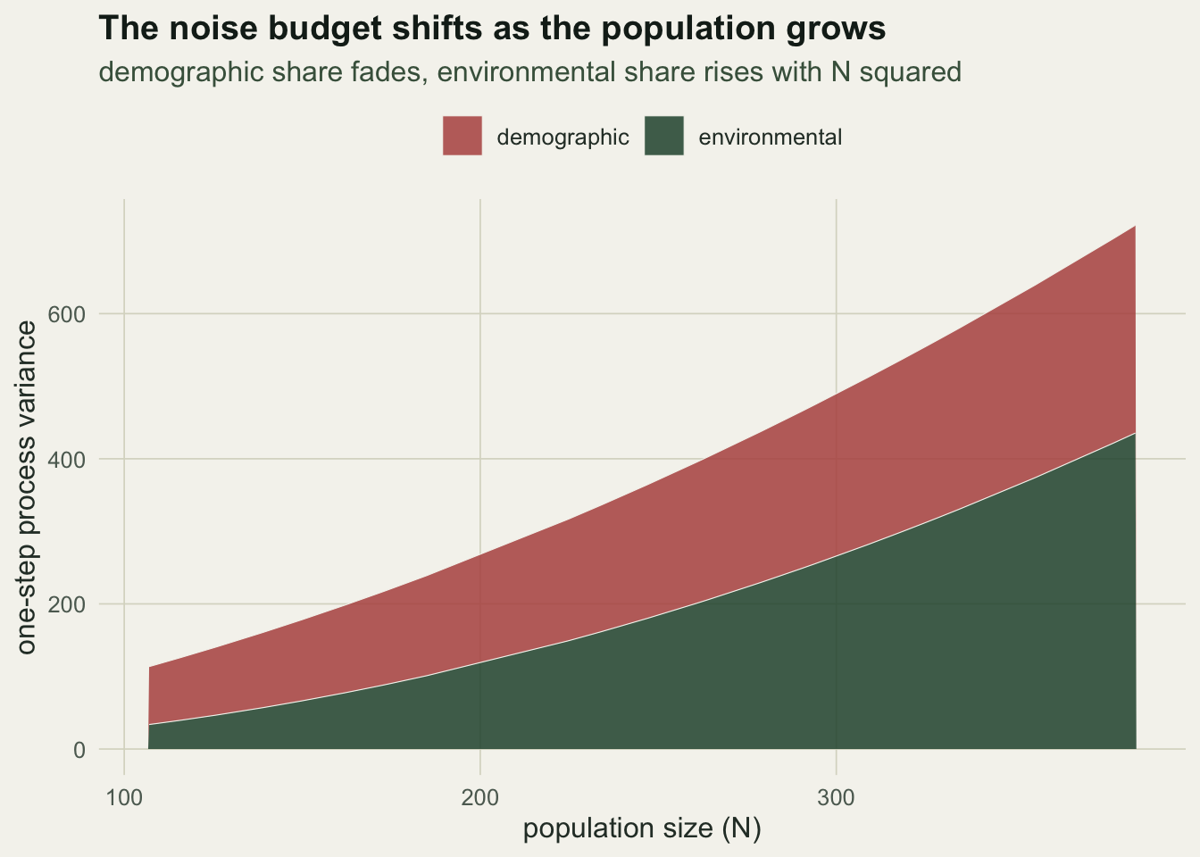
Dropping the demographic term pushes the environmental estimate to 0.077, about 1.41 times the value from the correct decomposition and well above the truth. The inflation seen here is modest because the population is fairly large; in a population of a few dozen it would be far larger. The point is structural: demographic noise mistaken for environmental noise makes a population look more at the mercy of the environment than it is. Tracing the two absolute variance terms along the trajectory shows the handover as the population grew.

lam <- phi_h + f_h
ap <- Pp <- af <- Pf <- numeric(Tyr); a <- exp(of$par[6]); P <- (2 * exp(of$par[4]))^2
for (t in 1:Tyr) {
  if (t > 1) { a <- lam * af[t - 1]; P <- lam^2 * Pf[t - 1] + dv_h * max(af[t - 1], 1) + se2_h * max(af[t - 1], 1)^2 }
  ap[t] <- a; Pp[t] <- P
  Fk <- P + exp(of$par[4])^2; K <- P / Fk
  af[t] <- a + K * (C[t] - a); Pf[t] <- (1 - K) * P
}
as_ <- af
for (t in (Tyr - 1):1) { J <- Pf[t] * lam / Pp[t + 1]; as_[t] <- af[t] + J * (as_[t + 1] - ap[t + 1]) }
dd <- data.frame(N = as_,
                 demographic = dv_h * as_,
                 environmental = se2_h * as_^2)
dd <- dd[order(dd$N), ]
dl <- rbind(data.frame(N = dd$N, v = dd$demographic, part = "demographic"),
            data.frame(N = dd$N, v = dd$environmental, part = "environmental"))
ggplot(dl, aes(N, v, fill = part)) +
  geom_area(alpha = 0.85, colour = paper, linewidth = 0.2) +
  scale_fill_manual(values = c(demographic = rust, environmental = forest), name = NULL) +
  labs(x = "population size (N)", y = "one-step process variance",
       title = "The noise budget shifts as the population grows",
       subtitle = "demographic share fades, environmental share rises with N squared") +
  theme_te() + theme(legend.position = "top")

Figure 2: Absolute process variance split into its demographic and environmental parts along the fitted trajectory, ordered by abundance. Early on, when numbers were low, demographic variance made up most of the process noise; as the population grew, the environmental term (which rises with the square of abundance) took over. The stack is the total one-step process variance the model attributes to each year.

Takeaways

Demographic and environmental variability are not interchangeable: one is the sampling noise of a finite population and fades as one over abundance, the other is the variation of the vital rates and holds steady, and which matters depends on how large the population is. An integrated model separates them because the capture-recapture and productivity data fix the vital rates, and so fix how much demographic scatter to expect; the leftover count variation is the environmental part. Two cautions travel with this. The environmental variance is estimated from the spread of a few dozen years and is never sharp, so its interval will be wide even when the point estimate is reasonable. And the separation only works if abundance varies enough to expose the different scalings; a population held near constant size over a short series leaves the two terms confounded. The final post in the series turns from estimation to checking: how to tell whether the data sets an integrated model combines actually agree.

References

Besbeas, P., Freeman, S. N., Morgan, B. J. T. and Catchpole, E. A. 2002. Integrating mark-recapture-recovery and census data to estimate animal abundance and demographic parameters. Biometrics 58(3):540-547 (10.1111/j.0006-341X.2002.00540.x).

Engen, S., Bakke, O. and Islam, A. 1998. Demographic and environmental stochasticity: concepts and definitions. Biometrics 54(3):840-846 (10.2307/2533838).

Lande, R., Engen, S. and Saether, B.-E. 2003. Stochastic Population Dynamics in Ecology and Conservation. Oxford University Press (ISBN 978-0-19-852525-7).

Saether, B.-E. and Engen, S. 2015. The concept of fitness in fluctuating environments. Trends in Ecology and Evolution 30(5):273-281 (10.1016/j.tree.2015.03.007).

Schaub, M. and Abadi, F. 2011. Integrated population models: a novel analysis framework for deeper insights into population dynamics. Journal of Ornithology 152(S1):227-237 (10.1007/s10336-010-0632-7).

Kery, M. and Schaub, M. 2012. Bayesian Population Analysis using WinBUGS. Academic Press (ISBN 978-0-12-387020-9).

Related tutorials

• Integrated population models from scratch
• Implicit information in integrated models
• Stochastic population growth
• The Gompertz state-space model