library(ggplot2)

te_pal <- list(forest = "#275139", green = "#2f8f63", sage = "#93a87f",
               clay = "#b5534e", gold = "#cda23f", line = "#dad9ca",
               ink = "#16241d", paper = "#f5f4ee")

theme_te <- function() {
  theme_minimal(base_size = 12) +
    theme(panel.grid.minor = element_blank(),
          panel.grid.major = element_line(colour = "#e7e6dc"),
          plot.background = element_rect(fill = "#f5f4ee", colour = NA),
          panel.background = element_rect(fill = "#f5f4ee", colour = NA),
          plot.title = element_text(face = "bold", colour = te_pal$ink),
          axis.title = element_text(colour = "#2c3a31"))
}Stochastic dynamic programming for harvest
R
conservation
decision analysis
ecology tutorial
ggplot2
Derive an optimal harvest rule in R by stochastic dynamic programming, then measure what recruitment noise does to it and what a concave payoff does to it.
A stock assessment lands in November. What is due in January is not a catch but a rule, because the same question comes back every November for as long as the fishery exists, and whatever is taken this winter changes what there is to count next winter. A consequence table cannot hold that. The consequence of this year’s catch is next year’s state, so the row you pick today edits the table you will be reading a year from now.
The object that can hold it is a policy: a function from the stock you observe to the catch you take, worked out once and then applied every year. This tutorial derives one for a single harvested population by stochastic dynamic programming and then measures four things about it. Does it reproduce the rule that pencil and paper give in the case where pencil and paper work? What does recruitment noise do to it? How much does it beat three rules a manager could write down with no dynamic programming at all? And how much of its shape comes from the biology as against the shape of the curve that turns a landed tonne into a payoff? The last of those turns out to move the rule further than the noise does.
Three earlier posts stop short of this problem. Structured decision making in R builds a consequence table for one decision whose consequences are fixed. The expected value of information prices what reducing uncertainty would be worth before that decision is taken. Adaptive management and learning repeats the decision and updates model weights as monitoring arrives, but the system being managed does not move underneath the manager between decisions. Here it moves, and it moves because of what she did.
Two fisheries posts sit either side of this one. The theta-logistic model supplies the population dynamics used below. Checking a stock assessment runs a closed loop simulation of three harvest control rules that were written down in advance and compares them on equal terms. This post does the missing half: it derives the rule that such a comparison should be measured against, and then measures the gap. The gap is smaller than the machinery would suggest in one direction and much larger in another, and which is which depends on a choice that is not biological at all.
A stock, a decision every November, and a rule
The system is one harvested population on an annual cycle. At the start of the year the stock is some biomass in thousands of tonnes and is known exactly. The fishery takes a catch, leaving an escapement behind it. What escapes spawns and grows over the year, and the stock at the start of next year is the escapement put through a growth function and multiplied by a recruitment shock with mean one. The shock is lognormal, with a standard deviation of 0.3 on the log scale, drawn fresh each year and independent between years.
The growth function is the discrete time theta-logistic, which is the Ricker curve when theta is one and skews the production curve to the left when theta is below one. The objective is the sum of catches discounted at a factor of 0.95 a year, and the horizon is unbounded, which is the formal way of saying that no year is the last one.
Two parts of that are assumptions rather than estimates and they carry most of the weight. The growth parameters are set, not fitted, so nothing below inherits the uncertainty a real assessment would carry. And the timing matters: the manager sets the catch, and only then does the year’s recruitment shock happen. That ordering is a modelling choice about who knows what and when, and the central result of this post depends on it.
r_max   <- 0.8
k_cap   <- 100
theta_g <- 0.8
gam     <- 0.95
sig_base <- 0.3
x_max   <- 240
n_grid  <- 1201
n_node  <- 25
grid    <- seq(0, x_max, length.out = n_grid)

recruit   <- function(s) s * exp(r_max * (1 - (s / k_cap)^theta_g))
recruit_d <- function(s) exp(r_max * (1 - (s / k_cap)^theta_g)) *
  (1 - r_max * theta_g * (s / k_cap)^theta_g)

s_msy <- uniroot(function(s) recruit_d(s) - 1, c(1, k_cap), tol = 1e-12)$root
peak  <- optimize(recruit, c(0, x_max), maximum = TRUE)

round(c(growth_rate = r_max, carrying_capacity = k_cap, theta = theta_g,
        discount_factor = gam, recruitment_sd = sig_base,
        grid_points = n_grid, grid_step = grid[2] - grid[1], grid_top = x_max,
        noise_nodes = n_node), 4)
growth_rate carrying_capacity theta discount_factor
0.80 100.00 0.80 0.95
recruitment_sd grid_points grid_step grid_top
0.30 1201.00 0.20 240.00
noise_nodes
25.00 round(c(escapement_at_max_yield = s_msy,
maximum_sustained_yield = recruit(s_msy) - s_msy,
largest_possible_recruitment = peak$objective,
escapement_that_gives_it = peak$maximum), 4) escapement_at_max_yield maximum_sustained_yield
42.9103 20.6849
largest_possible_recruitment escapement_that_gives_it
111.3891 174.6928 Carrying capacity is 100 thousand tonnes. The escapement that maximises sustained yield is 42.9103 thousand tonnes, delivering 20.6849 thousand tonnes a year for ever, and the largest recruitment the population can produce in any single year is 111.3891 thousand tonnes, from an escapement of 174.6928. Those are properties of the growth curve alone. None of them is the answer to the management question, because none of them knows about discounting or about noise.
The rule you can write down before the computer starts
The deterministic version of this problem has a closed form, and it is worth having in hand before any code runs, because it is the only check available that does not come from the same program being checked.
Suppose there is no recruitment shock. Consider a policy that leaves escapement \(S\) every year, applied from a stock \(x\) above \(S\). It takes \(x - S\) this year, and then \(f(S) - S\) every year after that, for ever. Its discounted value is
\[J(S) = (x - S) + \frac{\gamma}{1 - \gamma}\left(f(S) - S\right).\]
Differentiate in \(S\), set to zero, and everything cancels except a marginal condition with two symbols in it: \(\gamma f'(S) = 1\). A tonne left in the water earns the discounted marginal growth it produces; a tonne landed earns one. Leave fish exactly up to the point where those are equal.
s_target_an <- uniroot(function(s) gam * recruit_d(s) - 1, c(1, k_cap), tol = 1e-12)$root
value_closed <- function(s, x0 = 100) (x0 - s) + gam / (1 - gam) * (recruit(s) - s)

round(c(escapement_target_analytic = s_target_an,
        stock_next_year_at_target = recruit(s_target_an),
        sustained_yield_at_target = recruit(s_target_an) - s_target_an,
        closed_form_value_at_100 = value_closed(s_target_an)), 4)
escapement_target_analytic stock_next_year_at_target
39.8139 60.4181
sustained_yield_at_target closed_form_value_at_100
20.6041 451.6645 round(c(target_below_max_yield_percent = 100 * (s_msy - s_target_an) / s_msy,
sustained_yield_given_up_percent =
100 * (1 - (recruit(s_target_an) - s_target_an) / (recruit(s_msy) - s_msy))), 4) target_below_max_yield_percent sustained_yield_given_up_percent
7.2159 0.3906 The condition puts the target at 39.8139 thousand tonnes, from which the stock rebuilds to 60.4181 by the next November, giving a sustained catch of 20.6041. Discounting has moved the target 7.2159 per cent below the escapement that maximises sustained yield, and the whole cost of that move is 0.3906 per cent of the sustained catch. The production curve is close to flat over that stretch. That flatness is not a curiosity here; it comes back in the contest between rules and it is the reason the contest ends the way it does.
s_seq <- seq(0, 120, length.out = 500)
curve_df <- data.frame(
  escapement = rep(s_seq, 2),
  biomass = c(recruit(s_seq), recruit(s_seq) - s_seq),
  what = factor(rep(c("Stock next November", "Sustained yield"), each = length(s_seq)),
                levels = c("Stock next November", "Sustained yield")))

ggplot(curve_df, aes(escapement, biomass, colour = what)) +
  geom_abline(intercept = 0, slope = 1, colour = te_pal$line, linewidth = 1) +
  geom_vline(xintercept = s_target_an, colour = te_pal$clay,
             linetype = "dashed", linewidth = 0.8) +
  geom_vline(xintercept = s_msy, colour = te_pal$gold,
             linetype = "dashed", linewidth = 0.8) +
  geom_line(linewidth = 1.1) +
  annotate("text", x = 36, y = 96, hjust = 1, size = 3.1, colour = "#2c3a31",
           label = "target from the\ndiscounted condition") +
  annotate("text", x = 47, y = 62, hjust = 0, size = 3.1, colour = "#2c3a31",
           label = "escapement that maximises\nsustained yield") +
  annotate("text", x = 104, y = 100, hjust = 0, size = 3.1, colour = "#7c8a80",
           label = "replacement") +
  scale_colour_manual(values = c(te_pal$forest, te_pal$green), name = NULL) +
  labs(x = "Escapement left after fishing (thousand tonnes)",
       y = "Thousand tonnes",
       title = "Discounting pulls the target below the yield maximising escapement") +
  theme_te() +
  theme(legend.position = "top")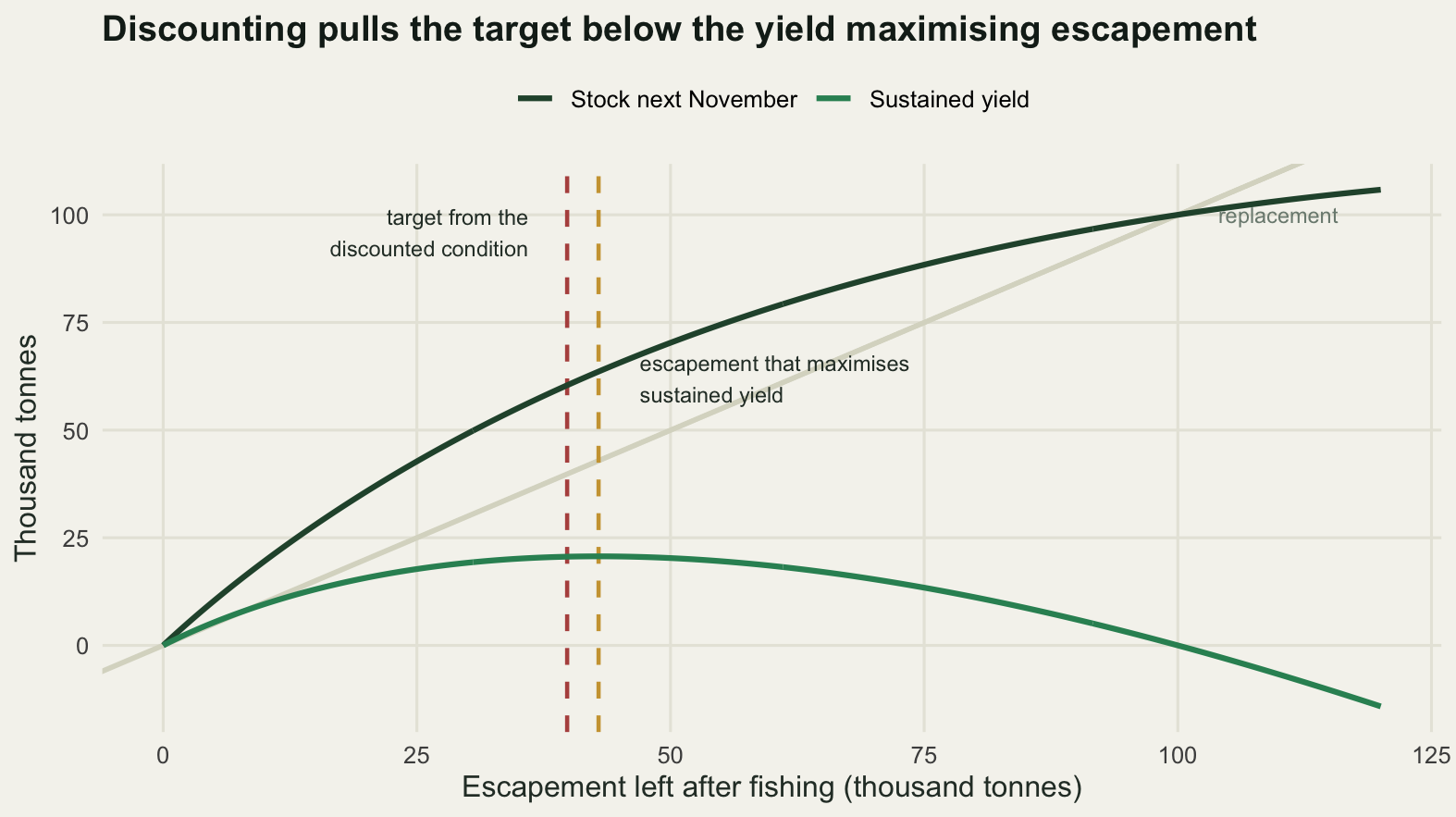
Solving the same problem backwards
The general problem is a Bellman equation. Write \(V(x)\) for the best achievable discounted payoff starting from stock \(x\), \(u\) for the payoff from a year’s catch, and \(z\) for the recruitment shock:
\[V(x) = \max_{0 \le s \le x}\left\{u(x - s) + \gamma\, \mathbb{E}\left[V\left(z f(s)\right)\right]\right\}.\]
Three approximations turn that into arithmetic. The stock is put on a grid of 1201 levels from 0 to 240 thousand tonnes, a spacing of 0.2. The shock is replaced by 25 equally likely nodes taken at the midpoints of its quantiles and then rescaled so that their mean is exactly one, which matters because a discretisation with a mean slightly off one is a different biological model. And \(V\) is interpolated linearly at the off-grid points \(z f(s)\) that the nodes land on.
Two solvers are written, for a reason that is itself part of the answer. When the payoff is linear in the catch, \(u(h) = h\), the objective splits: the terms in \(x\) and the terms in \(s\) come apart, and the best escapement to aim at stops depending on where you are starting from. The maximisation over all admissible escapements then collapses to a running maximum, which is one call to cummax. The second solver assumes nothing of the sort. It builds the full payoff matrix over every state and every admissible escapement and searches all of it, with a short policy evaluation loop inside each sweep to cut the number of expensive maximisations.
noise_nodes <- function(sig, m) {
  if (sig <= 0) return(rep(1, m))
  zr <- exp(sig * qnorm((seq_len(m) - 0.5) / m))
  zr / mean(zr)
}

ev_maker <- function(sig, m = n_node) {
  dx <- grid[2] - grid[1]
  y <- outer(recruit(grid), noise_nodes(sig, m))
  y[] <- pmin(pmax(y, 0), x_max)
  pos <- y / dx
  lo <- floor(pos)
  lo[lo > n_grid - 2] <- n_grid - 2
  wt <- as.numeric(pos - lo)
  lo <- as.integer(lo) + 1L
  om <- 1 - wt
  function(V) .rowMeans(V[lo] * om + V[lo + 1L] * wt, n_grid, m)
}

solve_escapement <- function(sig, tol = 1e-11, maxit = 4000) {
  evf <- ev_maker(sig)
  V <- numeric(n_grid); it <- 0; delta <- Inf
  while (delta > tol && it < maxit) {
    it <- it + 1
    gg <- gam * evf(V) - grid
    vn <- grid + cummax(gg)
    delta <- max(abs(vn - V)); V <- vn
  }
  gg <- gam * evf(V) - grid
  cm <- cummax(gg)
  list(V = V, esc = grid[match(cm, gg)], iter = it, resid = max(abs(grid + cm - V)))
}

solve_sdp <- function(sig, eta, tol = 1e-11, maxit = 400, inner = 20) {
  hh <- outer(grid, grid, "-")
  um <- matrix(-Inf, n_grid, n_grid)
  ok <- hh >= 0
  um[ok] <- hh[ok]^eta
  evf <- ev_maker(sig)
  rows <- seq_len(n_grid)
  V <- numeric(n_grid); it <- 0; delta <- Inf
  while (delta > tol && it < maxit) {
    it <- it + 1
    aa <- um + rep(gam * evf(V), each = n_grid)
    idx <- max.col(aa, ties.method = "first")
    vn <- aa[cbind(rows, idx)]
    ur <- um[cbind(rows, idx)]
    for (kk in seq_len(inner)) vn <- ur + gam * evf(vn)[idx]
    delta <- max(abs(vn - V)); V <- vn
  }
  aa <- um + rep(gam * evf(V), each = n_grid)
  idx <- max.col(aa, ties.method = "first")
  list(V = V, esc = grid[idx], iter = it, resid = max(abs(aa[cbind(rows, idx)] - V)))
}

zc <- noise_nodes(sig_base, n_node)
round(c(node_mean = mean(zc), lowest_node = min(zc), highest_node = max(zc),
        largest_reachable_stock = max(zc) * peak$objective), 4)
node_mean lowest_node highest_node
1.0000 0.5175 1.7744
largest_reachable_stock
197.6522 ev_err <- max(abs(ev_maker(sig_base)(grid) - recruit(grid)))
signif(c(expectation_error_on_a_linear_value = ev_err), 3)expectation_error_on_a_linear_value
5.68e-14 The expectation operator is checked on the one value function it can integrate exactly. If \(V(x) = x\) then the answer must be \(f(s)\,\mathbb{E}[z] = f(s)\), and the largest error over the whole grid is 5.68e-14. The nodes have a mean of exactly 1, the lowest sits at 0.5175 and the highest at 1.7744, so the largest stock reachable in one step is 197.6522 thousand tonnes, comfortably inside the grid ceiling of 240.
Now the calibration that matters: run the solver on the deterministic problem, where the answer is already known from the marginal condition.
det_fit <- solve_escapement(0)
i100 <- which(abs(grid - 100) < 1e-9)
above <- grid > 60
det_gap <- (value_closed(s_target_an) - det_fit$V[i100]) / value_closed(s_target_an)

round(c(sweeps = det_fit$iter,
        states_above_60 = sum(above),
        distinct_escapements_above_60 = length(unique(det_fit$esc[above])),
        numerical_target = det_fit$esc[n_grid],
        analytic_target = s_target_an,
        target_gap = abs(det_fit$esc[n_grid] - s_target_an)), 4)
sweeps states_above_60
553.0000 900.0000
distinct_escapements_above_60 numerical_target
1.0000 39.8000
analytic_target target_gap
39.8139 0.0139 signif(c(bellman_residual = det_fit$resid,
closure_branch_error = max(abs(det_fit$esc[grid < 39] - grid[grid < 39])),
relative_value_gap = det_gap), 3) bellman_residual closure_branch_error relative_value_gap
9.44e-12 0.00e+00 7.13e-08 round(c(numerical_value_at_100 = det_fit$V[i100],
closed_form_value_at_100 = value_closed(s_target_an)), 4) numerical_value_at_100 closed_form_value_at_100
451.6645 451.6645 The solve takes 553 sweeps to reach a Bellman residual of 9.44e-12. Across the 900 grid states above 60 thousand tonnes the policy takes exactly one distinct escapement value, 39.8, against the analytic 39.8139, which is inside the grid spacing of 0.2. Below the target the policy is escapement equals stock, catch nothing: across the states below 39 thousand tonnes the largest deviation from that is 0. The value at a stock of 100 is 451.6645 against the closed form’s 451.6645, a relative gap of 7.13e-08.
That is the shape people mean by constant escapement: fish down to a fixed level and stop, close the fishery when you are already below it. It is the answer to the deterministic problem, and it came out of a solver that was never told to look for it.
Recruitment noise moves the target and leaves the rule alone
The obvious guess is that noise ruins this. A fixed target looks like a rule for a world without surprises, and a manager facing variable recruitment might reasonably expect the optimal policy to hedge: fish a little harder when the stock is high, ease off when it is low, aim somewhere between the target and where you already are. Sweeping the recruitment standard deviation from 0 to 0.6 answers it directly.
sig_seq <- c(0, 0.1, 0.2, 0.3, 0.4, 0.5, 0.6)
sweep_fit <- lapply(sig_seq, solve_escapement)
sweep_tab <- t(sapply(seq_along(sig_seq), function(i) {
  z <- sweep_fit[[i]]
  c(recruitment_sd = sig_seq[i], target = z$esc[n_grid],
    distinct_targets_above_60 = length(unique(z$esc[above])),
    value_at_100 = z$V[i100])
}))
print(round(sweep_tab, 4))
recruitment_sd target distinct_targets_above_60 value_at_100
[1,] 0.0 39.8 1 451.6645
[2,] 0.1 39.8 1 451.6645
[3,] 0.2 39.8 1 451.6627
[4,] 0.3 40.2 1 451.0160
[5,] 0.4 40.8 1 448.2575
[6,] 0.5 41.6 1 442.0018
[7,] 0.6 42.6 1 431.1415round(c(target_rise_percent = 100 * (sweep_tab[7, 2] / sweep_tab[1, 2] - 1),
value_loss_percent = 100 * (1 - sweep_tab[7, 4] / sweep_tab[1, 4])), 4) target_rise_percent.target value_loss_percent.value_at_100
7.0352 4.5439 lin_fit <- sweep_fit[[4]]
gen_lin <- solve_sdp(sig_base, 1)
round(c(general_solver_sweeps = gen_lin$iter,
distinct_escapements_above_60 = length(unique(gen_lin$esc[above]))), 4) general_solver_sweeps distinct_escapements_above_60
31 1 val_diff <- max(abs(gen_lin$V - lin_fit$V))
signif(c(general_solver_residual = gen_lin$resid,
largest_value_difference = val_diff,
largest_escapement_difference = max(abs(gen_lin$esc - lin_fit$esc))), 3) general_solver_residual largest_value_difference
2.84e-13 1.74e-10
largest_escapement_difference
0.00e+00 The rule does not change shape at any noise level. At every standard deviation in the sweep the policy still takes exactly one escapement value across the 900 states above 60 thousand tonnes. What moves is the level, and it moves upward: 39.8 up to a standard deviation of 0.2, then 40.2 at 0.3, 41.6 at 0.5 and 42.6 at 0.6, a rise of 7.0352 per cent across the sweep. The value falls over the same range, from 451.6645 to 431.1415, a loss of 4.5439 per cent. Noise is expensive and it shifts the target a little; it does not make the rule state dependent.
This is not an artefact of the fast solver, though it would be a fair suspicion, since that solver exploits the separability that produces the answer. So the general solver, which searches every admissible escapement at every state and knows nothing about separability, was run at the same noise level with a linear payoff. It returns the same policy to the last grid point: the largest escapement difference over the 1201 states is 0 and the largest value difference is 1.74e-10.
The reason is a result of Reed’s from 1979 and it is short enough to state. With the payoff linear in the catch and the recruitment shock landing after the harvest decision, the value function is linear in the stock above the target, so the term the escapement controls carries no trace of the current stock. The best escapement is therefore the same at every stock high enough to reach it, whatever the noise does. Noise raises the target because in bad years the stock lands below it and the fishery closes, and a tonne in the water is worth more than a tonne landed on those occasions, which tilts the marginal condition upward.
What does bend the rule
Nothing so far has questioned whether a huge landing is worth its tonnage in the same way a small one is. The model assumed it, because the payoff has been the catch itself. Replace that with a concave payoff, \(u(h) = h^{0.6}\), which is what a fishery faces when a glut moves the price against it, and which is also the shape a manager gets by asking for steadier landings. Not one biological parameter changes.
eta_c <- 0.6
con_fit <- solve_sdp(sig_base, eta_c)
look <- c(10, 20, 30, 40, 60, 100, 160, 240)
li <- match(look, grid)
print(round(rbind(stock = look,
                  escapement_linear = lin_fit$esc[li],
                  escapement_concave = con_fit$esc[li],
                  catch_linear = look - lin_fit$esc[li],
                  catch_concave = look - con_fit$esc[li]), 4))
[,1] [,2] [,3] [,4] [,5] [,6] [,7] [,8]
stock 10.0 20.0 30.0 40.0 60.0 100.0 160.0 240.0
escapement_linear 10.0 20.0 30.0 40.0 40.2 40.2 40.2 40.2
escapement_concave 9.4 17.6 24.4 30.2 39.6 52.4 64.2 74.0
catch_linear 0.0 0.0 0.0 0.0 19.8 59.8 119.8 199.8
catch_concave 0.6 2.4 5.6 9.8 20.4 47.6 95.8 166.0round(c(payoff_exponent = eta_c, sweeps = con_fit$iter,
concave_escapement_lowest = min(con_fit$esc[above]),
concave_escapement_highest = max(con_fit$esc[above]),
concave_escapement_range = diff(range(con_fit$esc[above])),
linear_escapement_range = diff(range(lin_fit$esc[above])),
highest_closed_stock_linear = max(grid[lin_fit$esc == grid]),
highest_closed_stock_concave = max(grid[con_fit$esc == grid])), 4) payoff_exponent sweeps
0.6 30.0
concave_escapement_lowest concave_escapement_highest
39.6 74.0
concave_escapement_range linear_escapement_range
34.4 0.0
highest_closed_stock_linear highest_closed_stock_concave
40.2 3.4 signif(c(bellman_residual = con_fit$resid), 3)bellman_residual
2.56e-13 The policy is no longer flat anywhere. Across the 900 states above 60 thousand tonnes the concave escapement runs from 39.6 to 74.0, a range of 34.4 thousand tonnes, against a range of exactly 0 for the linear rule. At a stock of 240 the linear rule leaves 40.2 behind and the concave rule leaves 74.0. Fish are being banked: a tonne not landed in a bumper year is worth more when it is landed in a thin one, and the only thing that says so is the exponent.
The low end is the part worth staring at. The linear rule closes the fishery at every stock at or below 40.2 thousand tonnes. The concave rule closes it only at or below 3.4. At a stock of 20, well under the linear target, the linear policy lands nothing and the concave policy lands 2.4 thousand tonnes; at a stock of 10 it still lands 0.6. The mechanism is the exponent again, from the other side: with a power below one the marginal payoff of the first tonne landed is unbounded, so there is always something to be gained by landing a little, however thin the stock. A payoff curve chosen to make catches steadier has quietly abolished the closure.
rule_lab <- c("Linear payoff, no noise", "Linear payoff, sd 0.3", "Concave payoff, sd 0.3")
pol_df <- data.frame(
  stock = rep(grid, 3),
  escapement = c(sweep_fit[[1]]$esc, lin_fit$esc, con_fit$esc),
  rule = factor(rep(rule_lab, each = n_grid), levels = rule_lab))

flat_note <- paste0("flat target ",
                    format(sweep_fit[[1]]$esc[n_grid], nsmall = 1),
                    " with no noise, ",
                    format(lin_fit$esc[n_grid], nsmall = 1), " at sd 0.3")

ggplot(pol_df, aes(stock, escapement, colour = rule, linewidth = rule)) +
  geom_abline(intercept = 0, slope = 1, colour = te_pal$line, linewidth = 1) +
  geom_line() +
  annotate("text", x = 96, y = 108, hjust = 0, size = 3.1, colour = "#7c8a80",
           label = "no fishing") +
  annotate("segment", x = 150, xend = 150, y = 26, yend = 36.5,
           colour = te_pal$forest, linewidth = 0.4,
           arrow = arrow(length = unit(0.16, "cm"), type = "closed")) +
  annotate("text", x = 150, y = 21, hjust = 0.5, size = 3.1,
           colour = te_pal$forest, label = flat_note) +
  scale_colour_manual(values = c(te_pal$sage, te_pal$forest, te_pal$clay), name = NULL) +
  scale_linewidth_manual(values = c(3.2, 1.1, 1.2), name = NULL) +
  coord_cartesian(xlim = c(0, 240), ylim = c(0, 130)) +
  labs(x = "Stock observed in November (thousand tonnes)",
       y = "Escapement left after fishing",
       title = "Noise lifts the flat target; the payoff curve is what bends the rule") +
  theme_te() +
  theme(legend.position = "top")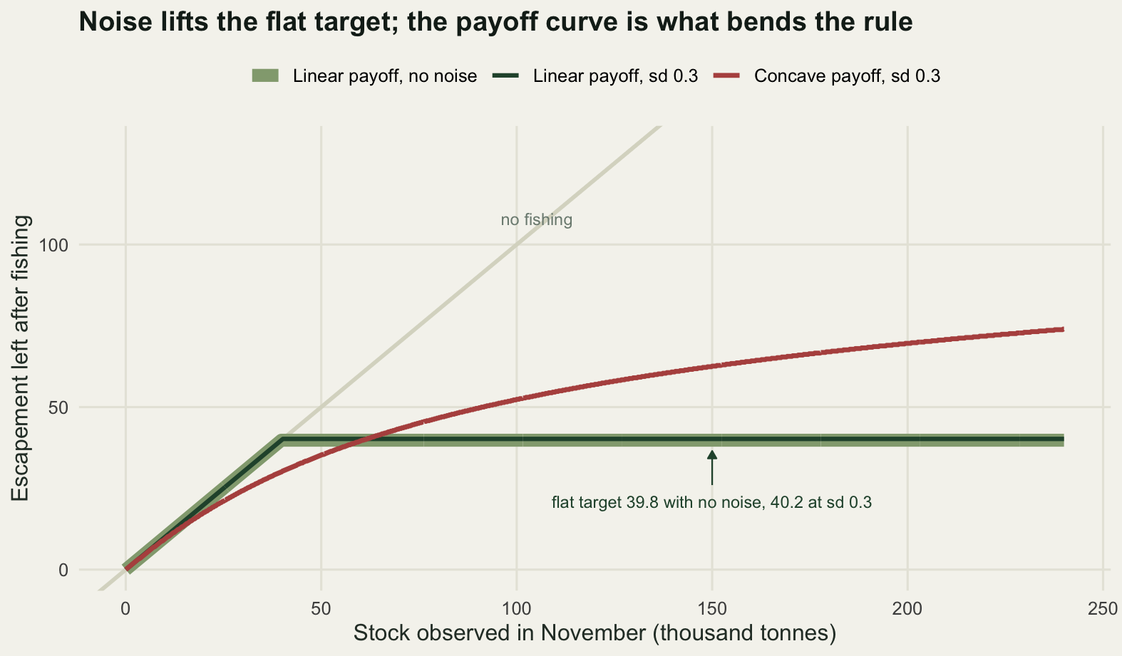
The optimum against three rules a manager could write down
An optimal policy is worth what it beats. The three rules below are the ones that get written down without any dynamic programming, and each is given every advantage. A constant harvest rate takes a fixed fraction of whatever is there. A fixed quota takes the same tonnage every year, or everything if less is available. A cut-off rule takes a fixed fraction of the stock above a threshold and nothing below it. Each family is tuned by grid search on the same simulated recruitment shocks that the comparison itself uses, with the true dynamics known, which is an advantage no real manager gets.
The simulator runs 4000 replicates of 60 years from a starting stock of 100 thousand tonnes, with common random numbers across every rule, so the comparisons are paired. Alongside the discounted catch it records the chance of the stock ever dropping below a limit reference point of 20 thousand tonnes, the fifth percentile of the discounted catch across replicates, the fraction of years with the fishery shut, and the average within-replicate coefficient of variation of the annual catch.
set.seed(20260722)
n_rep <- 4000; n_yr <- 60; x_start <- k_cap
zmat <- matrix(exp(sig_base * rnorm(n_rep * n_yr) - sig_base^2 / 2), n_rep, n_yr)
limit_ref <- 0.2 * k_cap
annuity <- (1 - gam^n_yr) / (1 - gam)
round(c(replicates = n_rep, years = n_yr, start_stock = x_start,
        limit_reference_point = limit_ref, realised_shock_mean = mean(zmat),
        discount_weight_on_last_year = gam^(n_yr - 1), annuity_factor = annuity), 5)
replicates years
4000.00000 60.00000
start_stock limit_reference_point
100.00000 20.00000
realised_shock_mean discount_weight_on_last_year
1.00087 0.04849
annuity_factor
19.07860 run_rule <- function(esc_fun, full = TRUE) {
xx <- rep(x_start, n_rep)
yld <- numeric(n_rep); utl <- numeric(n_rep)
low <- rep(FALSE, n_rep); shut <- numeric(n_rep)
csum <- numeric(n_rep); csq <- numeric(n_rep)
for (tt in seq_len(n_yr)) {
ss <- pmin(pmax(esc_fun(xx), 0), xx)
hh <- xx - ss
yld <- yld + gam^(tt - 1) * hh
xx <- recruit(ss) * zmat[, tt]
if (full) {
utl <- utl + gam^(tt - 1) * hh^eta_c
shut <- shut + (hh < 1e-9)
csum <- csum + hh; csq <- csq + hh^2
low <- low | (xx < limit_ref)
}
}
if (!full) return(list(yield = mean(yld)))
cbar <- csum / n_yr
list(yield = mean(yld), utility = mean(utl), risk = mean(low),
lower_fifth = as.numeric(quantile(yld, 0.05)), closed = mean(shut) / n_yr,
catch_cv = mean(sqrt(pmax(csq / n_yr - cbar^2, 0)) / pmax(cbar, 1e-9)),
yields = yld)
}
esc_sdp <- function(x) approx(grid, lin_fit$esc, x, rule = 2)$y
esc_concave <- function(x) approx(grid, con_fit$esc, x, rule = 2)$y
esc_rate <- function(phi) function(x) (1 - phi) * x
esc_quota <- function(cc) function(x) pmax(x - cc, 0)
esc_cutoff <- function(phi, xl) function(x) x - phi * pmax(x - xl, 0)
sdp_run <- run_rule(esc_sdp)
round(unlist(sdp_run[1:6]), 4) yield utility risk lower_fifth closed catch_cv
432.9539 110.2943 0.0203 341.8247 0.1192 0.8565 phi_seq <- seq(0.05, 0.75, by = 0.01)
rate_runs <- lapply(phi_seq, function(p) run_rule(esc_rate(p)))
rate_y <- sapply(rate_runs, function(z) z$yield)
rate_risk <- sapply(rate_runs, function(z) z$risk)
b_rate <- which.max(rate_y)
quota_seq <- seq(1, 40, by = 0.5)
quota_runs <- lapply(quota_seq, function(cc) run_rule(esc_quota(cc)))
quota_y <- sapply(quota_runs, function(z) z$yield)
quota_risk <- sapply(quota_runs, function(z) z$risk)
b_quota <- which.max(quota_y)
cut_grid <- expand.grid(phi = seq(0.4, 1, by = 0.05), xl = seq(20, 60, by = 2))
cut_y <- mapply(function(p, xl) run_rule(esc_cutoff(p, xl), full = FALSE)$yield,
cut_grid$phi, cut_grid$xl)
b_cut <- which.max(cut_y)
round(c(rate_settings_tried = length(phi_seq), quota_settings_tried = length(quota_seq),
cutoff_settings_tried = nrow(cut_grid), best_harvest_rate = phi_seq[b_rate],
best_quota = quota_seq[b_quota], best_cutoff_fraction = cut_grid$phi[b_cut],
best_cutoff_threshold = cut_grid$xl[b_cut]), 4) rate_settings_tried quota_settings_tried cutoff_settings_tried
71.00 79.00 273.00
best_harvest_rate best_quota best_cutoff_fraction
0.34 14.50 1.00
best_cutoff_threshold
40.00 best_rate <- rate_runs[[b_rate]]
best_quota <- quota_runs[[b_quota]]
best_cut <- run_rule(esc_cutoff(cut_grid$phi[b_cut], cut_grid$xl[b_cut]))
msy_run <- run_rule(function(x) pmin(x, s_msy))
con_run <- run_rule(esc_concave)
contest <- rbind(`optimal policy` = unlist(sdp_run[1:6]),
`best cut-off` = unlist(best_cut[1:6]),
`max yield escapement` = unlist(msy_run[1:6]),
`best harvest rate` = unlist(best_rate[1:6]),
`best fixed quota` = unlist(best_quota[1:6]),
`concave payoff policy` = unlist(con_run[1:6]))
print(round(contest, 4)) yield utility risk lower_fifth closed catch_cv
optimal policy 432.9539 110.2943 0.0203 341.8247 0.1192 0.8565
best cut-off 432.9560 110.3490 0.0205 342.0742 0.1181 0.8548
max yield escapement 431.7972 109.3393 0.0142 336.7952 0.1341 0.8802
best harvest rate 387.9830 113.5964 0.5290 300.6500 0.0000 0.4276
best fixed quota 213.2197 73.3128 0.8225 98.7442 0.4381 1.0426
concave payoff policy 422.5084 117.1902 0.1035 333.8552 0.0000 0.5992round(c(shortfall_percent = 100 * (1 - contest[, "yield"] / contest[1, "yield"])), 4) shortfall_percent.optimal policy shortfall_percent.best cut-off
0.0000 -0.0005
shortfall_percent.max yield escapement shortfall_percent.best harvest rate
0.2672 10.3870
shortfall_percent.best fixed quota shortfall_percent.concave payoff policy
50.7523 2.4126 paired <- function(a, b) c(mean_difference = mean(a$yields - b$yields),
standard_error = sd(a$yields - b$yields) / sqrt(n_rep))
print(round(rbind(`cut-off` = paired(sdp_run, best_cut),
`max yield escapement` = paired(sdp_run, msy_run),
`harvest rate` = paired(sdp_run, best_rate),
`fixed quota` = paired(sdp_run, best_quota)), 4)) mean_difference standard_error
cut-off -0.0021 0.0029
max yield escapement 1.1567 0.0383
harvest rate 44.9709 0.1540
fixed quota 219.7341 0.8449The optimal policy returns an expected discounted catch of 432.9539 thousand tonnes. The tuned cut-off rule returns 432.9560, which is 0.0005 per cent more, and the paired difference is -0.0021 with a standard error of 0.0029, so the two are indistinguishable in practice. That is not a coincidence and it is not a failure of the dynamic programming. The cut-off family contains the optimum: its best member turned out to be a fraction of 1.00 above a threshold of 40, which is constant escapement at 40 thousand tonnes written in different notation. A manager who guesses the right functional form and tunes it well has the optimal policy, and the dynamic programming has told her which form to guess.
Guessing the wrong form is expensive. The best constant harvest rate, 0.34 of the stock every year, returns 387.9830, which is 10.3870 per cent short, and the best fixed quota, 14.5 thousand tonnes a year, returns 213.2197, which is 50.7523 per cent short. Both paired differences are enormous relative to their standard errors. Fishing at the escapement that maximises sustained yield, 42.9103 rather than the optimum’s target, costs 0.2672 per cent: a paired difference of 1.1567 against a standard error of 0.0383, so it is a real loss and it is worth nothing.
Yield is only half of it, and the risk column is where the two simple rules give themselves away.
ok_rate <- which(rate_risk <= sdp_run$risk)
ok_quota <- which(quota_risk <= sdp_run$risk)
br <- ok_rate[which.max(rate_y[ok_rate])]
bq <- ok_quota[which.max(quota_y[ok_quota])]
round(c(risk_matched_rate = phi_seq[br], its_yield = rate_y[br], its_risk = rate_risk[br],
        its_shortfall_percent = 100 * (1 - rate_y[br] / sdp_run$yield),
        risk_matched_quota = quota_seq[bq], quota_yield = quota_y[bq],
        quota_risk = quota_risk[bq],
        quota_shortfall_percent = 100 * (1 - quota_y[bq] / sdp_run$yield)), 4)
risk_matched_rate its_yield its_risk
0.1700 266.7459 0.0185
its_shortfall_percent risk_matched_quota quota_yield
38.3893 6.5000 123.9592
quota_risk quota_shortfall_percent
0.0200 71.3690 tgt_seq <- seq(20, 70, by = 0.5)
tgt_y <- sapply(tgt_seq, function(s) run_rule(function(x) pmin(x, s), full = FALSE)$yield)
flat <- tgt_seq[tgt_y >= 0.99 * max(tgt_y)]
round(c(best_constant_escapement = tgt_seq[which.max(tgt_y)],
within_one_percent_from = min(flat), within_one_percent_to = max(flat),
width_of_that_band = diff(range(flat))), 4)best_constant_escapement within_one_percent_from within_one_percent_to
40.0 35.0 45.5
width_of_that_band
10.5 The optimal policy leaves the stock below 20 thousand tonnes at some point in the 60 years in 0.0203 of replicates. The tuned harvest rate does it in 0.5290 and the tuned quota in 0.8225. Those two rules bought their yield partly with risk, so compare them again with the risk held level. The best constant harvest rate whose collapse chance does not exceed the optimal policy’s is 0.17, and it returns 266.7459, which is 38.3893 per cent short. The best fixed quota under the same constraint is 6.5 thousand tonnes a year, returning 123.9592, or 71.3690 per cent short. So the gap between an optimal rule and a simple one is not the 10.3870 per cent that the comparison tuned for yield reports. It is the 38.3893 per cent that appears once the risk is held level, and the rest of it had been hiding in the risk column.
The other half of the same measurement points the other way. Constant escapement targets anywhere from 35.0 to 45.5 thousand tonnes, a band 10.5 wide around the best value of 40.0, are within one per cent of the best discounted catch that any target achieves. Getting the form of the rule right is worth tens of per cent. Getting the level right, given the form, is worth fractions of one. The flatness of the production curve seen in the first figure is what pays for that, and it is the practical argument for spending the effort on the structure of the rule rather than on the third decimal place of the target.
fam_df <- rbind(
  data.frame(risk = rate_risk, yield = rate_y, family = "Constant harvest rate"),
  data.frame(risk = quota_risk, yield = quota_y, family = "Fixed quota"))
pt_df <- data.frame(
  risk = c(sdp_run$risk, con_run$risk, best_rate$risk, best_quota$risk),
  yield = c(sdp_run$yield, con_run$yield, best_rate$yield, best_quota$yield),
  lab = c("optimal policy", "concave payoff policy", "best rate", "best quota"),
  hj = c(0, 0, 0.5, 0.5), vj = c(-1.3, 2.2, 2.1, 2.1))

ggplot(fam_df, aes(risk, yield)) +
  geom_path(aes(colour = family), linewidth = 1.1) +
  geom_point(data = pt_df, shape = 18, size = 4, colour = te_pal$ink) +
  geom_text(data = pt_df, aes(label = lab, hjust = hj, vjust = vj), size = 3.1,
            colour = "#2c3a31") +
  scale_colour_manual(values = c(te_pal$gold, te_pal$clay), name = NULL) +
  coord_cartesian(xlim = c(-0.03, 1.02), ylim = c(0, 470)) +
  labs(x = "Chance the stock drops below 20 thousand tonnes within 60 years",
       y = "Expected discounted catch (thousand tonnes)",
       title = "The simple rules pay for their catch in collapse risk") +
  theme_te() +
  theme(legend.position = "top")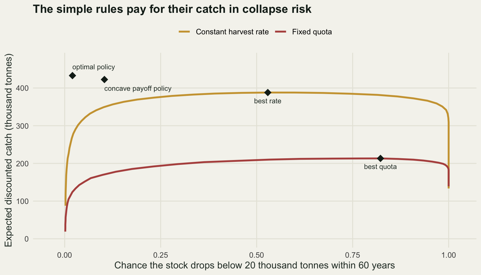
How much of the rule is the payoff curve
The payoff exponent was set to 0.6 without any argument for that number, which is exactly how such numbers usually get set. Sweeping it shows how much of the answer it is carrying.
eta_seq <- c(1, 0.85, 0.7, 0.55, 0.4)
eta_fit <- lapply(eta_seq, function(e) solve_sdp(sig_base, e))
eta_tab <- t(sapply(seq_along(eta_seq), function(i) {
  e <- eta_fit[[i]]$esc
  c(exponent = eta_seq[i], escapement_at_50 = e[match(50, grid)],
    escapement_at_100 = e[match(100, grid)], escapement_at_200 = e[match(200, grid)],
    range_above_60 = diff(range(e[above])), catch_at_stock_20 = 20 - e[match(20, grid)])
}))
print(round(eta_tab, 4))
exponent escapement_at_50 escapement_at_100 escapement_at_200
[1,] 1.00 40.2 40.2 40.2
[2,] 0.85 37.0 46.4 53.8
[3,] 0.70 35.6 50.4 63.8
[4,] 0.55 35.0 53.2 72.2
[5,] 0.40 34.6 55.6 79.6
range_above_60 catch_at_stock_20
[1,] 0.0 0.0
[2,] 15.8 0.4
[3,] 27.6 1.8
[4,] 37.6 2.8
[5,] 46.4 3.6At an exponent of 1 the rule is flat: 40.2 at every stock, a range of 0. Bend the payoff a little, to 0.85, and the escapement is already 37.0 at a stock of 50 and 53.8 at a stock of 200, and across the states above 60 it spans 15.8 thousand tonnes. At 0.4 it is 34.6 at a stock of 50 and 79.6 at a stock of 200, and the span above 60 widens to 46.4. The catch taken at a stock of 20, which the linear rule refuses to touch at all, climbs from 0 through 0.4, 1.8 and 2.8 to 3.6 thousand tonnes as the exponent falls. Every one of those five rules is optimal. They are optimal for five different statements about what a landed tonne is worth, and the population model underneath them is identical.
eta_df <- do.call(rbind, lapply(seq_along(eta_seq), function(i)
  data.frame(stock = grid, escapement = eta_fit[[i]]$esc,
             exponent = factor(format(eta_seq[i], nsmall = 2),
                               levels = format(eta_seq, nsmall = 2)))))

ggplot(eta_df, aes(stock, escapement, colour = exponent)) +
  geom_abline(intercept = 0, slope = 1, colour = te_pal$line, linewidth = 1) +
  geom_line(linewidth = 1.1) +
  scale_colour_manual(values = c(te_pal$forest, te_pal$green, te_pal$sage,
                                 te_pal$gold, te_pal$clay),
                      name = "Payoff exponent") +
  coord_cartesian(xlim = c(0, 240), ylim = c(0, 130)) +
  labs(x = "Stock observed in November (thousand tonnes)",
       y = "Escapement left after fishing",
       title = "One population model, five payoff curves, five different rules") +
  theme_te() +
  theme(legend.position = "right")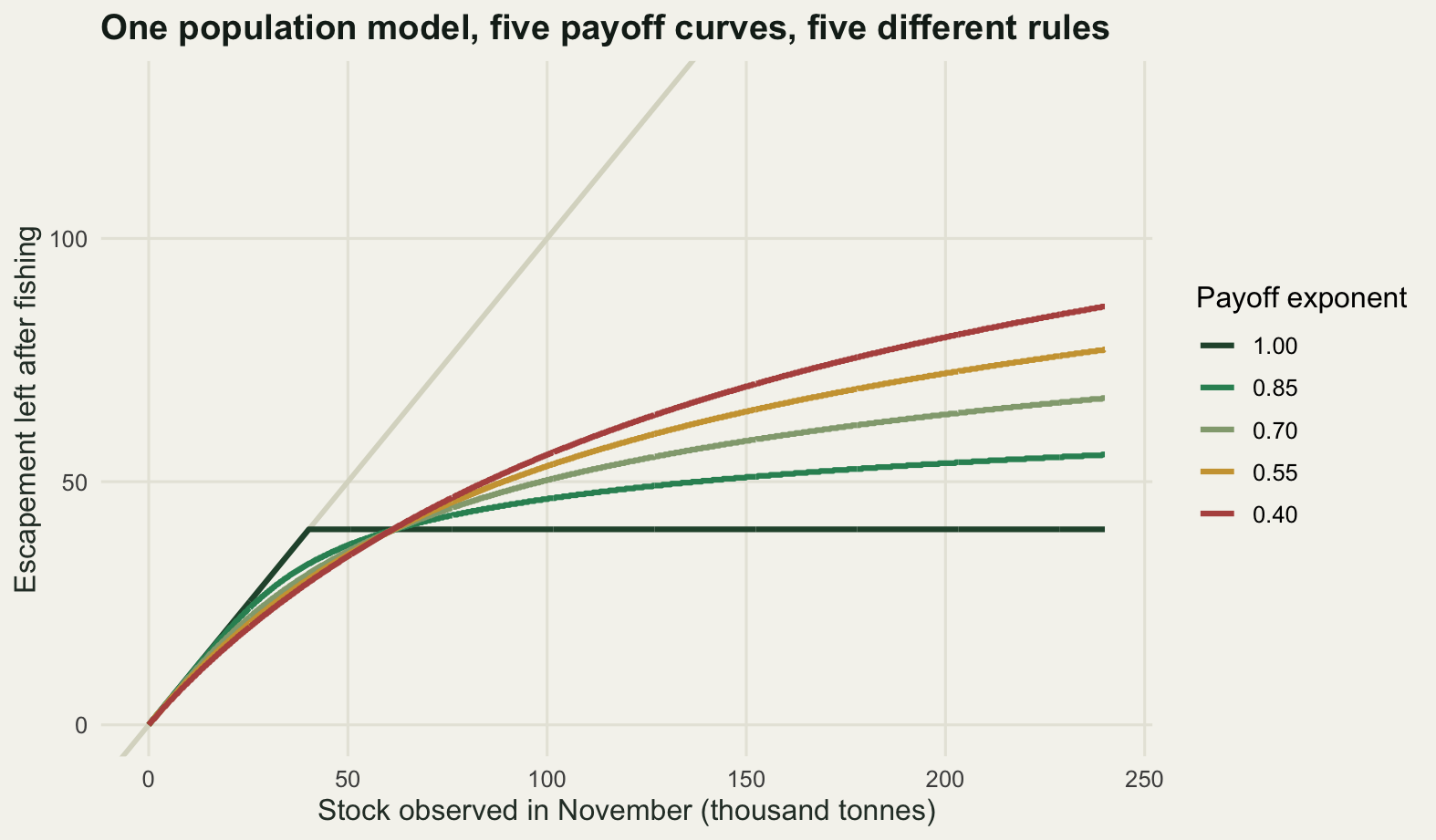
Two of those rules can be put on the simulator and made to argue. Run the linear policy and the concave policy through the same 4000 replicates and score both under both objectives. To make the payoff comparable to tonnes, convert the discounted payoff into the constant annual catch that would deliver the same total, by dividing by the annuity factor of 19.0786 and undoing the exponent.
ce <- function(u) (u / annuity)^(1 / eta_c)
cross <- rbind(`linear policy` = c(sdp_run$yield, sdp_run$utility, ce(sdp_run$utility),
                                   sdp_run$risk, sdp_run$catch_cv, sdp_run$closed),
               `concave policy` = c(con_run$yield, con_run$utility, ce(con_run$utility),
                                    con_run$risk, con_run$catch_cv, con_run$closed))
colnames(cross) <- c("yield", "payoff", "equivalent_catch", "risk", "catch_cv", "closed")
print(round(cross, 4))
yield payoff equivalent_catch risk catch_cv closed
linear policy 432.9539 110.2943 18.6213 0.0203 0.8565 0.1192
concave policy 422.5084 117.1902 20.6019 0.1035 0.5992 0.0000round(c(catch_lost_by_the_concave_policy_percent = 100 * (1 - cross[2, 1] / cross[1, 1]),
equivalent_catch_lost_by_the_linear_policy_percent =
100 * (1 - cross[1, 3] / cross[2, 3]),
risk_multiple = cross[2, 4] / cross[1, 4]), 4) catch_lost_by_the_concave_policy_percent
2.4126
equivalent_catch_lost_by_the_linear_policy_percent
9.6136
risk_multiple
5.1111 Each policy wins on its own objective, which is the least it could do. Judged in tonnes the concave policy gives up 2.4126 per cent of the discounted catch. Judged in equivalent annual catch under the concave payoff the linear policy gives up 9.6136 per cent, 18.6213 thousand tonnes a year against 20.6019. It also does what it was asked to do about steadiness: the coefficient of variation of the annual catch falls from 0.8565 to 0.5992, and the fishery is never shut, against 0.1192 of years shut under the linear rule.
Then the column nobody asked for. The chance of the stock dropping below 20 thousand tonnes rises from 0.0203 under the linear policy to 0.1035 under the concave one, a factor of 5.1111. The rule that produces steadier landings and never closes the fishery is about five times more likely to run the stock into the ground. It is the same mechanism as the abolished closure: a payoff curve that makes the first tonne of a small catch enormously valuable will keep fishing a collapsing stock, and it will do so while reporting a smoother catch series than the alternative. If a management strategy evaluation compares the two on catch and catch variability, which is the usual pair, the concave rule wins on both and the risk it is carrying appears in neither.
The honest limit
The transition model is assumed, not estimated. Growth rate, carrying capacity, theta and the recruitment standard deviation were set by hand, and none of the uncertainty in them is in the state. Every measurement above is a statement about the rule you should follow if that model is true, and the machinery here has nothing to say about the far more common situation in which it is not. Putting parameter uncertainty into the state is the step from this post to adaptive management and learning, and it changes the size of the problem, not just its answers.
The stock is observed without error and the catch is taken without error. Both are large assumptions in a real fishery, and both work in the direction of flattering the optimal policy, which fishes exactly to a target that it can see exactly. The closed loop with assessment error and implementation error in it is a different measurement.
The timing is a choice. The recruitment shock lands after the harvest decision, so the manager never has to commit to a catch before knowing what she is cutting into. Reed’s result depends on that ordering. Set the catch before the shock resolves and the constant escapement result weakens, which is one reason real advice is more cautious than the rule derived here.
The discount factor of 0.95 is not a parameter of the fish. It moved the target 7.2159 per cent below the yield maximising escapement all by itself, and a manager who prefers a different figure is making an ethical and financial argument, not a biological one. The same goes for the payoff exponent, with more force: the sweep over exponents measured how much of the rule it carries.
The grid resolves escapement to 0.2 thousand tonnes and the state space stops at 240, and the simulator truncates at 60 years, which discards the tail beyond a discount weight of 0.04849. The simple rules were tuned on the same shocks the comparison used, which flatters them slightly; the optimal policy was not tuned at all. And the collapse risk quoted throughout is a modelled quantity, computed against a limit reference point of 20 thousand tonnes that was chosen here rather than negotiated with anyone.
Where to go next
The obvious next question is what happens when the state has to be estimated rather than observed, which is where checking a stock assessment picks up: the same closed loop, with an assessment model in the middle of it and the rules taking their input from that rather than from the truth. Going the other way, into the machinery itself, markov decision processes for management sets out the discrete state version of everything above, where the transition matrix is written out in full and the Bellman equation can be solved by linear algebra.
The diagnostics that this post did not run are collected in checking a sequential decision model: what the grid spacing is doing to the answer, what the discount factor is doing to it, how much a transition model fitted to a short series of observations costs against one that is known, and how far the end of a finite horizon reaches back into the policy.
References
Reed WJ 1979 Journal of Environmental Economics and Management 6(4):350-363 (10.1016/0095-0696(79)90014-7)
Marescot L, Chapron G, Chades I, Fackler PL, Duchamp C, Marboutin E, Gimenez O 2013 Methods in Ecology and Evolution 4(9):872-884 (10.1111/2041-210X.12082)
Walters CJ, Hilborn R 1978 Annual Review of Ecology and Systematics 9:157-188 (10.1146/annurev.es.09.110178.001105)
Clark CW 2010 Mathematical Bioeconomics: The Mathematics of Conservation, 3rd edition. Wiley, ISBN 978-0-470-37299-9
Hilborn R, Walters CJ 1992 Quantitative Fisheries Stock Assessment: Choice, Dynamics and Uncertainty. Chapman and Hall, ISBN 978-0-412-02271-5