library(ggplot2)

te_pal <- list(forest = "#275139", green = "#2f8f63", sage = "#93a87f",
               clay = "#b5534e", gold = "#cda23f", line = "#dad9ca",
               ink = "#16241d", paper = "#f5f4ee")

theme_te <- function() {
  theme_minimal(base_size = 12) +
    theme(panel.grid.minor = element_blank(),
          panel.grid.major = element_line(colour = "#e7e6dc"),
          plot.background = element_rect(fill = "#f5f4ee", colour = NA),
          panel.background = element_rect(fill = "#f5f4ee", colour = NA),
          plot.title = element_text(face = "bold", colour = te_pal$ink),
          axis.title = element_text(colour = "#2c3a31"))
}Adaptive management and learning
R
conservation
decision analysis
ecology tutorial
ggplot2
Two hypotheses about harvest mortality in a hunted population, Bayesian model weights updated each year, and the horizon at which active management pays off.
A wildlife agency has to publish a hunting regulation every autumn. Two accounts of what the hunting does have been argued over for half a century. Under the additive account, every bird taken is a bird that would otherwise have been alive next spring. Under the compensatory account, hunting removes birds that were going to die of something else anyway, and up to some harvest rate the spring population does not notice. The two accounts recommend opposite regulations, and the data an agency holds are usually too thin to separate them.
The obvious way forward is to act on your current best guess and update the guess from what happens. That is passive adaptive management, and its failure is not statistical. The information a year of monitoring carries depends on which regulation you set, because the two hypotheses only disagree about what harvest does. Set a token season and both hypotheses predict the same count next spring, so the count tells you nothing, so you set a token season again. The scheme is stable, defensible in a meeting, and permanently ignorant.
Active adaptive management takes the other side of that trade: set a regulation that looks worse under your current beliefs, because the separation it buys is worth more than the birds it costs. The claim is only worth making if the crossover can be measured. This post builds the whole apparatus by hand: a population with two candidate harvest responses, five regulations, a spring survey with a stated error, and a Bayesian update of the model weights from each year’s count. Then it measures the learning rate under each regulation, prices the conflict between what pays and what teaches, and reports the year at which the active scheme overtakes the passive one.
The decision structure itself, an objective and an action set and a set of states, is taken as given here; Structured decision making in R builds one from nothing. What this post adds is the year to year update, and the part of the problem that only appears once the manager is allowed to act more than once.
A population, two hypotheses and five regulations
The state is the spring breeding population, in thousands of birds. Recruitment is Ricker, so the autumn flight is the spring population multiplied by an exponential term that falls with crowding. Harvest takes a fraction of that flight, and the kill is what the agency counts as yield. What happens to the rest over winter is where the two hypotheses part company.
Write the annual survival multiplier as a function of the harvest rate, scaled so that it equals one when nothing is shot. The additive hypothesis subtracts the kill one for one. The compensatory hypothesis leaves survival untouched while the harvest rate stays under a threshold, on the grounds that the shot birds come entirely out of a doomed surplus, and becomes additive again above it once that surplus is exhausted.
Next spring’s population is the harvested flight times the survival multiplier, times a lognormal process deviation. The manager never sees it. The spring survey returns the population times a lognormal error with a standard deviation of 0.06 on the log scale, against a process standard deviation of 0.10.
The objective needs saying out loud, because it decides everything that follows. Maximising the kill alone would always recommend the heaviest available season, and no agency manages that way. The value of a year here is the kill, plus 2.5 units for every bird by which the spring population exceeds carrying capacity and minus the same for every bird it falls short. A bird left standing is worth two and a half birds in the bag. That one number carries the population goal a real regulation is written against.
Two things are assumed known: the growth rate and the carrying capacity. The uncertainty is deliberately confined to the harvest response. Everything measured below about learning is therefore optimistic, because a real programme is uncertain about its recruitment as well.
K <- 100
r_grow <- 0.6
comp_thr <- 0.20
part_comp <- 0.35
bird_value <- 2.5
sig_proc <- 0.10
sig_obs <- 0.06
sig_pred <- sqrt(sig_proc^2 + sig_obs^2)
actions <- c(0.02, 0.05, 0.10, 0.18, 0.30)
horizon <- 60
prior_comp <- 0.35
nrep <- 600
nrep_c <- 800

phi_add  <- function(h) 1 - h
phi_comp <- function(h) ifelse(h <= comp_thr, 1, (1 - h) / (1 - comp_thr))
phi_part <- function(h) 1 - part_comp * h
flight   <- function(n) n * exp(r_grow * (1 - n / K))
reward   <- function(h, p, n1) h * p + bird_value * (n1 - K)

d_act <- log(phi_comp(actions)) - log(phi_add(actions))
kl_act <- d_act^2 / (2 * sig_pred^2)

round(c(carrying_capacity = K, growth_rate = r_grow,
        compensation_threshold = comp_thr, bird_value = bird_value,
        process_sd = sig_proc, survey_sd = sig_obs, predictive_sd = sig_pred,
        horizon_years = horizon, prior_on_compensation = prior_comp,
        partial_compensation = part_comp,
        replicates = nrep, learning_replicates = nrep_c), 5)
carrying_capacity growth_rate compensation_threshold
100.00000 0.60000 0.20000
bird_value process_sd survey_sd
2.50000 0.10000 0.06000
predictive_sd horizon_years prior_on_compensation
0.11662 60.00000 0.35000
partial_compensation replicates learning_replicates
0.35000 600.00000 800.00000 print(round(rbind(harvest_per_cent = 100 * actions,
survival_if_additive = phi_add(actions),
survival_if_compensatory = phi_comp(actions),
log_ratio = d_act,
kl_per_year = kl_act,
years_to_0.9_predicted = log(9) / kl_act), 4)) [,1] [,2] [,3] [,4] [,5]
harvest_per_cent 2.0000 5.0000 10.0000 18.0000 30.0000
survival_if_additive 0.9800 0.9500 0.9000 0.8200 0.7000
survival_if_compensatory 1.0000 1.0000 1.0000 1.0000 0.8750
log_ratio 0.0202 0.0513 0.1054 0.1985 0.2231
kl_per_year 0.0150 0.0967 0.4081 1.4479 1.8306
years_to_0.9_predicted 146.4280 22.7155 5.3838 1.5175 1.2003Read the bottom three rows. The log ratio is the gap between what the two hypotheses predict for next spring’s log count, and it grows from 0.0202 under a 2 per cent season to 0.2231 under a 30 per cent one. Divide that gap by the predictive standard deviation of 0.11662, square it and halve it, and you have the Kullback-Leibler divergence between the two predictive distributions. That quantity is also the expected log Bayes factor one year of the regulation delivers in favour of whichever hypothesis is true, and it runs from 0.0150 to 1.8306. The last row turns it into years: starting from an even prior, the heaviest season needs 1.2003 years to push the weight on the truth to 0.9, and the lightest needs 146.4280.
Two features of that table are worth holding on to. The compensatory survival is exactly 1 for the first four regulations and 0.8750 for the fifth, so if compensation holds then the first four seasons are free. And the information saturates, though not yet at 30 per cent: above the compensation threshold of 20 per cent the two hypotheses run parallel, differing by the constant factor 1 / 0.8, so every regulation heavier than that separates them at the same rate of 1.8306 a year while costing steadily more population.
Does the updater find the truth?
The update is the standard one. At the start of a year the manager holds a weight on the compensatory hypothesis. It reads the survey count, projects the autumn flight from it, and forms a prediction of next spring’s log count under each hypothesis. Next spring’s survey arrives, each hypothesis gets a normal likelihood with standard deviation 0.11662, and the weights are multiplied by their likelihoods and renormalised. The arithmetic is done in log odds, which stays stable when one hypothesis is being crushed.
There is an approximation in that predictive standard deviation. It combines the process and survey errors but ignores the fact that the starting count was itself observed with error, which propagates through the projection. Rather than argue about whether that matters, we measure it: standardise the one step residuals under the hypothesis that actually generated the data, and check that they have mean zero and unit spread. The validation run holds the 10 per cent season constant for 60 years, once with each hypothesis true, starting from the manager’s prior weight of 0.35 on compensation.
run_constant <- function(h, truth_phi, nrep, nyr, seed) {
  set.seed(seed)
  n <- rep(K, nrep)
  lo <- rep(log(prior_comp / (1 - prior_comp)), nrep)
  obs <- n * exp(rnorm(nrep, 0, sig_obs))
  keep <- res <- res_c <- matrix(0, nyr, nrep)
  la <- log(phi_add(h)); lc <- log(phi_comp(h)); lt <- log(truth_phi(h))
  for (t in seq_len(nyr)) {
    p <- flight(n)
    n <- pmax(p * truth_phi(h) * exp(rnorm(nrep, 0, sig_proc)), 1e-6)
    obs_new <- n * exp(rnorm(nrep, 0, sig_obs))
    pred <- log(obs) + r_grow * (1 - obs / K)
    lo <- pmax(-200, pmin(200, lo +
      dnorm(log(obs_new), pred + lc, sig_pred, log = TRUE) -
      dnorm(log(obs_new), pred + la, sig_pred, log = TRUE)))
    keep[t, ] <- lo
    res[t, ] <- (log(obs_new) - (pred + lt)) / sig_pred
    res_c[t, ] <- (log(obs_new) - (pred + lc)) / sig_pred
    obs <- obs_new
  }
  list(lo = keep, res = res, res_c = res_c)
}

runs_c <- lapply(seq_along(actions), function(j)
  run_constant(actions[j], phi_comp, nrep_c, horizon, 1100 + j))
runs_a <- lapply(seq_along(actions), function(j)
  run_constant(actions[j], phi_add, nrep_c, horizon, 1200 + j))

wc10 <- plogis(runs_c[[3]]$lo)
wa10 <- plogis(-runs_a[[3]]$lo)
round(c(comp_true_year5 = mean(wc10[5, ]), comp_true_year10 = mean(wc10[10, ]),
        comp_true_year25 = mean(wc10[25, ]),
        comp_years_to_median_0.9 = which(apply(wc10, 1, median) > 0.9)[1],
        add_true_year5 = mean(wa10[5, ]), add_true_year10 = mean(wa10[10, ]),
        add_true_year25 = mean(wa10[25, ]),
        add_years_to_median_0.9 = which(apply(wa10, 1, median) > 0.9)[1]), 4)
comp_true_year5 comp_true_year10 comp_true_year25
0.7160 0.8625 0.9825
comp_years_to_median_0.9 add_true_year5 add_true_year10
7.0000 0.8540 0.9312
add_true_year25 add_years_to_median_0.9
0.9890 4.0000 round(c(resid_mean_comp = mean(runs_c[[3]]$res),
resid_sd_comp = sd(as.vector(runs_c[[3]]$res)),
resid_mean_add = mean(runs_a[[3]]$res),
resid_sd_add = sd(as.vector(runs_a[[3]]$res))), 4)resid_mean_comp resid_sd_comp resid_mean_add resid_sd_add
0.0071 1.0143 0.0108 1.0370 The updater works. With compensation true, the mean weight on compensation climbs from 0.35 to 0.7160 by year 5, 0.8625 by year 10 and 0.9825 by year 25, and the median replicate passes 0.9 in year 7. With additive mortality true, the mean weight on additive reaches 0.8540, 0.9312 and 0.9890 at the same three points and the median crosses in year 4. The additive case is quicker only because the prior already leans that way, which is what a precautionary prior is for.
The residual check returns a mean of 0.0071 and a standard deviation of 1.0143 when compensation is true, and 0.0108 and 1.0370 when additive mortality is true. The predictive standard deviation is slightly too small, by roughly the amount the ignored survey error in the starting count contributes, and the effect is small enough to leave alone. A larger discrepancy would matter a great deal, because weights that move too fast are the standard way a Bayesian model comparison talks itself into a wrong answer.
Learning is a property of the action
Now the part that matters. Hold each of the five regulations constant for 60 years, under both truths, and record how far the weights get. Nothing about the estimator changes between runs. Only the regulation changes.
learn_tab <- t(sapply(seq_along(actions), function(j) {
  wc <- plogis(runs_c[[j]]$lo)
  wa <- plogis(-runs_a[[j]]$lo)
  yc <- which(apply(wc, 1, median) > 0.9)[1]
  ya <- which(apply(wa, 1, median) > 0.9)[1]
  c(harvest_per_cent = 100 * actions[j], kl_per_year = kl_act[j],
    mean_weight_year20 = prior_comp * mean(wc[20, ]) +
      (1 - prior_comp) * mean(wa[20, ]),
    log_bayes_factor_year20 = prior_comp * mean(runs_c[[j]]$lo[20, ]) +
      (1 - prior_comp) * mean(-runs_a[[j]]$lo[20, ]),
    years_if_comp_true = yc, years_if_add_true = ya)
}))
print(round(learn_tab, 4))
harvest_per_cent kl_per_year mean_weight_year20 log_bayes_factor_year20
[1,] 2 0.0150 0.6017 0.4770
[2,] 5 0.0967 0.7908 2.0525
[3,] 10 0.4081 0.9767 8.2452
[4,] 18 1.4479 1.0000 29.0337
[5,] 30 1.8306 1.0000 36.9004
years_if_comp_true years_if_add_true
[1,] NA NA
[2,] 29 17
[3,] 7 4
[4,] 2 2
[5,] 2 1round(c(prior_weight_on_true_model = prior_comp^2 + (1 - prior_comp)^2,
spearman_kl_vs_learning =
cor(learn_tab[, "kl_per_year"],
learn_tab[, "log_bayes_factor_year20"], method = "spearman")), 4)prior_weight_on_true_model spearman_kl_vs_learning
0.545 1.000 Averaged over which hypothesis is true, the prior already puts 0.545 on the true model. After 20 years of a 2 per cent season that has moved to 0.6017, and the median replicate never reaches 0.9 inside the horizon under either truth. The predicted requirement was 146.4280 years, so this is not a shortage of replicates; it is a regulation under which the two hypotheses are very nearly the same model. A 5 per cent season needs 29 years if compensation is true and 17 if additive mortality is; a 10 per cent season needs 7 and 4; the two heaviest need 2 years, or 1.
The mean log posterior odds on the true hypothesis after 20 years ranks the regulations 0.4770, 2.0525, 8.2452, 29.0337 and 36.9004, and its Spearman correlation with the divergence is 1. That ranking is arithmetic rather than discovery: for two normal predictions sharing a variance the expected log Bayes factor per year is exactly the divergence, and 20 years of it comes to 0.3001, 1.9346, 8.1624, 28.9579 and 36.6125. Those five are evidence alone, while the printed column, despite its label, starts from the manager’s prior odds and carries them, which over the two truths, weighted 0.35 to compensation, adds the same constant to every entry: 0.1857. Add it to those five predictions and the printed values land on them, a little to either side, which is Monte Carlo scatter rather than a shift. The 2 per cent season is where it shows, because the constant is the same size under every regulation: a large share of the 0.4770 printed there and a rounding error against the 36.9004 at 30 per cent. What the simulation adds beyond the ranking is the spread, which the divergence does not carry.
The information does have a ceiling, but it does not fall between these two regulations. Going from 18 to 30 per cent buys 36.9004 against 29.0337, a quarter more evidence for a season two thirds heavier, and the population pays the whole difference. The ceiling sits above the compensation threshold of 20 per cent, where the two survival curves differ by the constant factor 1 / 0.8: the log ratio is pinned at 0.2231 and the divergence at 1.8306 however heavy the season gets, so a 50 per cent harvest would teach at exactly the rate a 30 per cent one does and cost far more. The 18 per cent season sits just below the threshold, which is why the step to 30 still buys something. Where an experiment stops paying for itself is a property of the hypotheses rather than of the manager’s nerve.
lab_act <- paste0(round(100 * actions), " per cent")
trace <- do.call(rbind, lapply(seq_along(actions), function(j) rbind(
  data.frame(year = seq_len(horizon),
             weight = rowMeans(plogis(runs_c[[j]]$lo)),
             regulation = lab_act[j], truth = "Compensation is true"),
  data.frame(year = seq_len(horizon),
             weight = rowMeans(plogis(-runs_a[[j]]$lo)),
             regulation = lab_act[j], truth = "Additive mortality is true"))))
trace$regulation <- factor(trace$regulation, levels = lab_act)
trace$truth <- factor(trace$truth,
                      levels = c("Compensation is true", "Additive mortality is true"))

ggplot(trace, aes(year, weight, colour = regulation)) +
  geom_hline(yintercept = 0.9, colour = te_pal$line, linewidth = 0.7,
             linetype = "22") +
  geom_line(linewidth = 0.8) +
  facet_wrap(~truth) +
  scale_colour_manual(values = c(te_pal$sage, te_pal$gold, te_pal$green,
                                 te_pal$forest, te_pal$clay),
                      name = "Harvest rate") +
  coord_cartesian(ylim = c(0, 1)) +
  labs(x = "Year", y = "Weight on the true hypothesis",
       title = "The regulation decides how fast the manager learns") +
  theme_te() +
  theme(legend.position = "top",
        strip.text = element_text(colour = te_pal$ink, face = "bold"))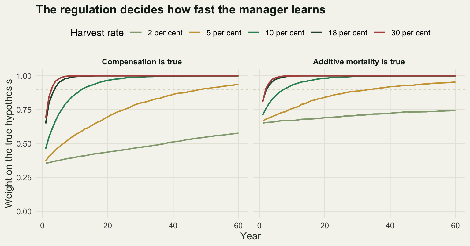
The regulation that pays best is the one that teaches you nothing
So heavier seasons teach faster. If heavier seasons also paid better there would be no post. Evaluate one year of each regulation with the population sitting at carrying capacity and the weights at the prior.
one_year <- function(h, phi_f, n0 = K) {
  p <- flight(n0)
  reward(h, p, p * phi_f(h))
}
ret_comp <- sapply(actions, one_year, phi_f = phi_comp)
ret_add <- sapply(actions, one_year, phi_f = phi_add)
ret_prior <- prior_comp * ret_comp + (1 - prior_comp) * ret_add

print(round(rbind(harvest_per_cent = 100 * actions,
                  return_if_compensatory = ret_comp,
                  return_if_additive = ret_add,
                  expected_return_under_prior = ret_prior,
                  kl_per_year = kl_act), 4))
[,1] [,2] [,3] [,4] [,5]
harvest_per_cent 2.000 5.0000 10.0000 18.0000 30.0000
return_if_compensatory 2.000 5.0000 10.0000 18.0000 -1.2500
return_if_additive -3.000 -7.5000 -15.0000 -27.0000 -45.0000
expected_return_under_prior -1.250 -3.1250 -6.2500 -11.2500 -29.6875
kl_per_year 0.015 0.0967 0.4081 1.4479 1.8306round(c(spearman_return_vs_kl = cor(ret_prior, kl_act, method = "spearman"),
pearson_return_vs_kl = cor(ret_prior, kl_act),
best_action_under_prior_pct = 100 * actions[which.max(ret_prior)],
most_informative_action_pct = 100 * actions[which.max(kl_act)]), 4) spearman_return_vs_kl pearson_return_vs_kl
-1.0000 -0.9043
best_action_under_prior_pct most_informative_action_pct
2.0000 30.0000 Under compensation the return climbs with the season, 2, 5, 10 and 18, then falls to -1.25 at 30 per cent where the compensation runs out and the population starts paying. Under additive mortality it falls the whole way, from -3 to -45. Averaged over the prior the expected return is -1.25, -3.1250, -6.2500, -11.2500 and -29.6875, which is monotone decreasing. The best regulation under the prior is the 2 per cent season and the most informative is the 30 per cent one. The Spearman correlation between expected return and information is -1, and the Pearson correlation is -0.9043.
Every one of those expected returns is negative, which is not a coding error. With the population goal set at carrying capacity and most of the prior weight on harvest being additive, any season is expected to cost more in birds left standing than it returns in birds shot. The manager is choosing between losses. What matters is that the ordering of the losses is the exact reverse of the ordering of the information.
That is the trap, stated precisely. A manager who each year picks the regulation maximising expected return under current beliefs picks the 2 per cent season, and the 2 per cent season is the one under which the median weight on the truth never reaches 0.9 in 60 years. The scheme is not failing to learn because the statistics are weak. It is failing to learn because it keeps choosing not to run the experiment.
conf <- data.frame(ret = ret_prior, kl = kl_act, lab = lab_act,
                   dx = c(0.9, -0.6, 0, 0, 0),
                   dy = c(0, -0.12, 0.12, 0.12, 0.12),
                   hj = c(0, 1, 0.5, 0.5, 0.5))

ggplot(conf, aes(ret, kl)) +
  geom_line(colour = te_pal$line, linewidth = 1) +
  geom_point(colour = te_pal$forest, size = 3.2) +
  geom_text(aes(x = ret + dx, y = kl + dy, label = lab, hjust = hj),
            colour = te_pal$ink, size = 3.4) +
  coord_cartesian(xlim = c(-33, 5), ylim = c(-0.18, 2.15)) +
  labs(x = "Expected one year return under the prior",
       y = "Information per year (KL divergence)",
       title = "Return and information pull in opposite directions",
       subtitle = "Each point is one regulation, labelled by its harvest rate") +
  theme_te() +
  theme(plot.subtitle = element_text(colour = "#2c3a31"))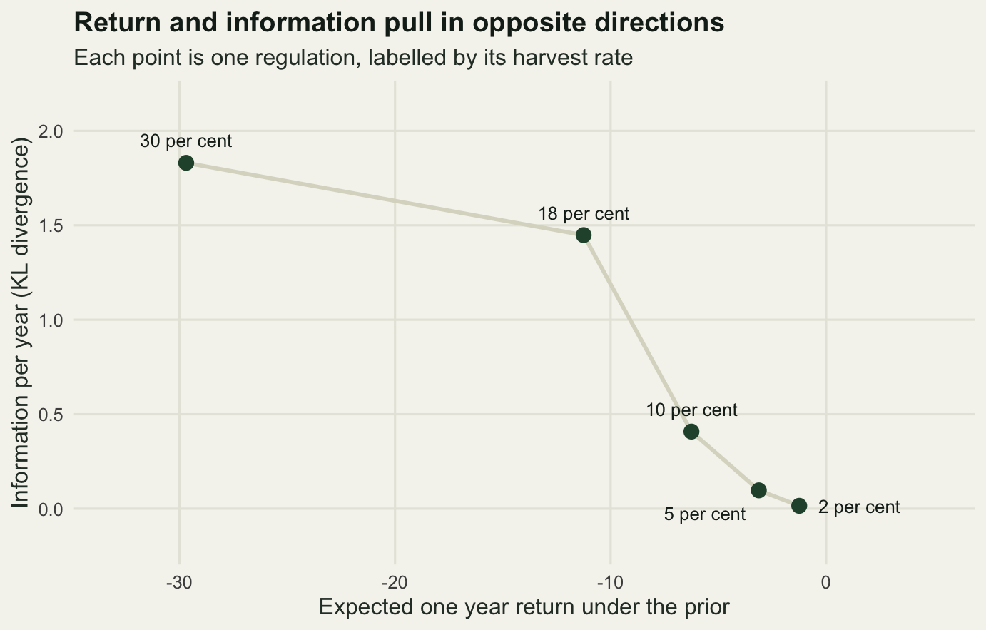
Paying for information on purpose
Two schemes, sharing an estimator and an action set.
The passive manager treats the current weights as correct and permanent. Each year it takes its observed count, rolls every regulation forward deterministically to the end of the horizon under each hypothesis, averages the two totals by the current weights, and takes the best. That is what acting as if the current best model were true amounts to when the current belief is a mixture: the belief enters the valuation and is then assumed never to change again.
The active manager evaluates the same regulations in two stages. Stage one is this year’s expected return. Stage two lets this year’s survey arrive, updates the weights, and then takes the best constant regulation for the remaining years under the updated weights. The expectation over possible surveys is a quadrature on the standardised observation. There is no tuning constant anywhere: the price the scheme will pay for information is whatever the improved second stage decision turns out to be worth.
That construction understates the value of information, because it allows exactly one round of learning and then freezes the belief for the rest of the horizon. The full problem is a dynamic program over the belief state, and its solution would experiment at least as much as this one does. The crossover below is a conservative estimate rather than a best case.
Both schemes run against both truths on common random numbers, so the survey and process deviations are identical across schemes until the schemes actually choose differently. The true hypothesis is drawn from the manager’s own prior, which puts 0.35 on compensation. That is the comparison a decision analysis is entitled to make.
roll <- function(n0, h, phi_f, steps) {
  n <- n0
  tot <- numeric(length(n0))
  for (s in seq_len(steps)) {
    p <- flight(n)
    n <- p * phi_f(h)
    tot <- tot + reward(h, p, n)
  }
  tot
}
row_max <- function(M) {
  r <- M[, 1]
  for (j in 2:ncol(M)) r <- pmax(r, M[, j])
  r
}
zq <- seq(-4, 4, length.out = 15)
c(quadrature_points = length(zq))
quadrature_points
15 run_policy <- function(mode, truth_phi, nrep, nyr, seed) {
set.seed(seed)
n <- rep(K, nrep)
lo <- rep(log(prior_comp / (1 - prior_comp)), nrep)
obs <- n * exp(rnorm(nrep, 0, sig_obs))
ret <- act <- pop <- lom <- res_c <- matrix(0, nyr, nrep)
nact <- length(actions)
for (t in seq_len(nyr)) {
w <- plogis(lo)
w1 <- plogis(-lo)
win <- nyr - t + 1
Vc <- Va <- matrix(0, nrep, nact)
for (j in seq_len(nact)) {
Vc[, j] <- roll(obs, actions[j], phi_comp, win)
Va[, j] <- roll(obs, actions[j], phi_add, win)
}
if (mode == "passive") {
j <- max.col(w * Vc + w1 * Va, ties.method = "first")
} else {
score <- matrix(0, nrep, nact)
for (jj in seq_len(nact)) {
h <- actions[jj]
p0 <- flight(obs)
n1a <- p0 * phi_add(h)
n1c <- p0 * phi_comp(h)
first <- w * reward(h, p0, n1c) + w1 * reward(h, p0, n1a)
Cc <- Ca <- matrix(0, nrep, nact)
if (win > 1) for (b in seq_len(nact)) {
Cc[, b] <- roll(n1c, actions[b], phi_comp, win - 1)
Ca[, b] <- roll(n1a, actions[b], phi_add, win - 1)
}
dl <- d_act[jj] / sig_pred
pa <- dnorm(zq)
pc <- dnorm(zq - dl)
tot <- wsum <- numeric(nrep)
for (k in seq_along(zq)) {
qk <- w1 * pa[k] + w * pc[k]
wk <- plogis(pmax(-25, pmin(25, lo + dl * zq[k] - dl^2 / 2)))
tot <- tot + qk * row_max(wk * Cc + (1 - wk) * Ca)
wsum <- wsum + qk
}
score[, jj] <- first + tot / wsum
}
j <- max.col(score, ties.method = "first")
}
h <- actions[j]
p <- flight(n)
n <- pmax(p * truth_phi(h) * exp(rnorm(nrep, 0, sig_proc)), 1e-6)
ret[t, ] <- reward(h, p, n)
act[t, ] <- h
pop[t, ] <- n
obs_new <- n * exp(rnorm(nrep, 0, sig_obs))
pred <- log(obs) + r_grow * (1 - obs / K)
res_c[t, ] <- (log(obs_new) - (pred + log(phi_comp(h)))) / sig_pred
lo <- pmax(-25, pmin(25, lo +
dnorm(log(obs_new), pred + log(phi_comp(h)), sig_pred, log = TRUE) -
dnorm(log(obs_new), pred + log(phi_add(h)), sig_pred, log = TRUE)))
lom[t, ] <- lo
obs <- obs_new
}
list(ret = ret, act = act, pop = pop, lo = lom, res_c = res_c)
}
pas_c <- run_policy("passive", phi_comp, nrep, horizon, 101)
pas_a <- run_policy("passive", phi_add, nrep, horizon, 102)
act_c <- run_policy("active", phi_comp, nrep, horizon, 101)
act_a <- run_policy("active", phi_add, nrep, horizon, 102)
cum_pc <- apply(pas_c$ret, 2, cumsum); cum_pa <- apply(pas_a$ret, 2, cumsum)
cum_ac <- apply(act_c$ret, 2, cumsum); cum_aa <- apply(act_a$ret, 2, cumsum)
mix <- function(x, y) prior_comp * rowMeans(x) + (1 - prior_comp) * rowMeans(y)
cum_pas <- mix(cum_pc, cum_pa)
cum_act <- mix(cum_ac, cum_aa)
cross <- which(cum_act > cum_pas)[1]
yrs <- c(5, 15, 30, 60)
print(round(rbind(passive = cum_pas[yrs], active = cum_act[yrs],
gap = (cum_act - cum_pas)[yrs]), 2)) [,1] [,2] [,3] [,4]
passive -6.86 -39.00 -85.38 -162.90
active -35.73 -27.61 -3.88 38.57
gap -28.87 11.39 81.50 201.47print(round(rbind(passive_if_compensatory = rowMeans(cum_pc)[yrs],
active_if_compensatory = rowMeans(cum_ac)[yrs],
passive_if_additive = rowMeans(cum_pa)[yrs],
active_if_additive = rowMeans(cum_aa)[yrs]), 2)) [,1] [,2] [,3] [,4]
passive_if_compensatory 16.16 37.56 78.32 237.53
active_if_compensatory 86.86 244.24 488.52 984.06
passive_if_additive -19.26 -80.22 -173.52 -378.52
active_if_additive -101.74 -173.99 -269.01 -470.55round(c(crossover_year = cross, deficit_at_year5 = cum_pas[5] - cum_act[5],
active_gain_if_compensatory = rowMeans(cum_ac)[horizon] -
rowMeans(cum_pc)[horizon],
active_loss_if_additive = rowMeans(cum_pa)[horizon] -
rowMeans(cum_aa)[horizon]), 3) crossover_year deficit_at_year5
13.000 28.872
active_gain_if_compensatory active_loss_if_additive
746.531 92.027 set.seed(5)
boot <- replicate(300, {
i1 <- sample(nrep, replace = TRUE)
i2 <- sample(nrep, replace = TRUE)
g <- prior_comp * (rowMeans(cum_ac[, i1]) - rowMeans(cum_pc[, i1])) +
(1 - prior_comp) * (rowMeans(cum_aa[, i2]) - rowMeans(cum_pa[, i2]))
c(which(g > 0)[1], g[5])
})
round(c(crossover_boot_lo = quantile(boot[1, ], 0.05, names = FALSE),
crossover_boot_hi = quantile(boot[1, ], 0.95, names = FALSE),
deficit5_boot_lo = -quantile(boot[2, ], 0.95, names = FALSE),
deficit5_boot_hi = -quantile(boot[2, ], 0.05, names = FALSE)), 3)crossover_boot_lo crossover_boot_hi deficit5_boot_lo deficit5_boot_hi
12.000 14.000 27.070 31.146 wmix <- function(rc, ra, yr) prior_comp * mean(plogis(rc$lo[yr, ])) +
(1 - prior_comp) * mean(plogis(-ra$lo[yr, ]))
w_inf <- prior_comp * mean(plogis(runs_c[[4]]$lo[horizon, ])) +
(1 - prior_comp) * mean(plogis(-runs_a[[4]]$lo[horizon, ]))
round(c(passive_weight_year60 = wmix(pas_c, pas_a, horizon),
active_weight_year60 = wmix(act_c, act_a, horizon),
informative_action_weight_year60 = w_inf,
weight_gap = w_inf - wmix(pas_c, pas_a, horizon)), 4) passive_weight_year60 active_weight_year60
0.7358 0.9381
informative_action_weight_year60 weight_gap
1.0000 0.2642 amix <- function(rc, ra) 100 * (prior_comp * rowMeans(rc$act) +
(1 - prior_comp) * rowMeans(ra$act))
print(round(rbind(passive_mean_harvest_pct = amix(pas_c, pas_a)[c(1, 2, 5, 20, 60)],
active_mean_harvest_pct = amix(act_c, act_a)[c(1, 2, 5, 20, 60)]), 4)) [,1] [,2] [,3] [,4] [,5]
passive_mean_harvest_pct 2 2.0000 2.0000 2.0653 4.9627
active_mean_harvest_pct 18 9.7373 7.0893 6.9333 7.0027The passive manager opens with the 2 per cent season and is still on it twenty years later, at a mean of 2.0653 per cent, and has crept only to 4.9627 per cent by year 60. The active manager opens with the 18 per cent season in every single replicate, drops to a mean of 9.7373 per cent by year 2 and settles near 7 per cent once it knows what it is dealing with.
The cost arrives first. At year 5 the passive scheme has accumulated -6.86 and the active scheme -35.73, a deficit of 28.872, with a bootstrap over replicates putting that between 27.070 and 31.146. By year 15 the active scheme is 11.39 ahead. The crossover is year 13, bootstrapped between 12 and 14. By year 30 the gap is 81.50 and by year 60 it is 201.47.
Splitting by which hypothesis was true shows where the money comes from. If compensation is true the active scheme ends on 984.06 against 237.53 for the passive one, a gain of 746.531. If additive mortality is true it ends on -470.55 against -378.52, a loss of 92.027. Weight those two by the prior and you recover the 201.47. The active scheme is buying a small and fairly reliable loss in the world where the precautionary hypothesis holds, in exchange for a large gain in the world where it does not.
One asymmetry should be stated plainly, because it flatters the active scheme. Under compensation the informative regulation and the profitable regulation are the same regulation: if harvest is free then harvesting hard is both the experiment and the payoff. The whole cost of the experiment falls in the additive branch. That is not a quirk of these parameters, it is what the compensatory hypothesis means, but it does mean the active scheme does better here than it would in a problem where the informative action is bad under every hypothesis.
The weights at the end tell the same story from the other side. After 60 years the passive scheme’s mean weight on the true hypothesis is 0.7358 and the active scheme’s is 0.9381. The 18 per cent season held constant reaches 1.0000, a gap of 0.2642 over the passive scheme. The passive manager is not frozen: it drifts, and by year 60 it has drifted far enough to start liberalising. It simply spends most of a working career not knowing.
cum_df <- rbind(
  data.frame(year = seq_len(horizon), value = cum_pas, scheme = "Passive"),
  data.frame(year = seq_len(horizon), value = cum_act, scheme = "Active"))

ggplot(cum_df, aes(year, value, colour = scheme)) +
  geom_hline(yintercept = 0, colour = te_pal$line, linewidth = 0.7) +
  geom_vline(xintercept = cross, colour = te_pal$gold, linewidth = 0.7,
             linetype = "22") +
  geom_line(linewidth = 0.9) +
  scale_colour_manual(values = c(Passive = te_pal$clay, Active = te_pal$forest),
                      name = NULL) +
  labs(x = "Year", y = "Cumulative return",
       title = paste0("Active management overtakes passive in year ", cross)) +
  theme_te() +
  theme(legend.position = "top")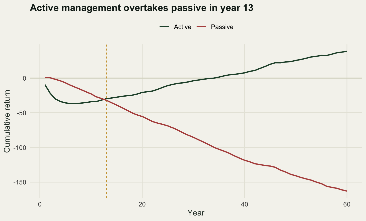
The honest limit: the truth has to be in the set
Everything above rests on an assumption that nothing inside the scheme ever tests: one of the two hypotheses is true. Bayesian model weights are relative. They say which of the models you wrote down fits better. They say nothing about whether either of them fits.
So generate the data from a third harvest response that is in neither hypothesis. Let a fixed fraction of harvest mortality be compensated at every rate, with no threshold and no saturation, by setting the survival multiplier to one minus 0.35 times the harvest rate. It is not the additive model and it is not the compensatory one. Under the four lighter regulations it lies between the two, and at 30 per cent it passes above the compensatory curve, at 0.8950 against 0.8750. At every harvest rate in the action set it sits closer to the compensatory hypothesis than to the additive one.
out_const <- run_constant(0.18, phi_part, nrep_c, horizon, 3001)
in_const <- run_constant(0.18, phi_comp, nrep_c, horizon, 3002)
w_out <- plogis(out_const$lo)
round(c(weight_on_compensatory_year30 = mean(w_out[30, ]),
        weight_on_compensatory_year60 = mean(w_out[60, ]),
        median_weight_year60 = median(w_out[60, ]),
        per_cent_above_0.9 = 100 * mean(w_out[60, ] > 0.9),
        weight_when_truth_is_in_set = mean(plogis(in_const$lo[60, ]))), 4)
weight_on_compensatory_year30 weight_on_compensatory_year60
0.9583 0.9938
median_weight_year60 per_cent_above_0.9
1.0000 98.8750
weight_when_truth_is_in_set
1.0000 out_pol <- run_policy("active", phi_part, nrep, horizon, 205)
bench <- sapply(actions, function(h) {
set.seed(900)
n <- rep(K, nrep)
tot <- numeric(nrep)
for (t in seq_len(horizon)) {
p <- flight(n)
n <- pmax(p * phi_part(h) * exp(rnorm(nrep, 0, sig_proc)), 1e-6)
tot <- tot + reward(h, p, n)
}
mean(tot) / horizon
})
print(round(rbind(harvest_per_cent = 100 * actions,
annual_return_under_truth = bench), 4)) [,1] [,2] [,3] [,4] [,5]
harvest_per_cent 2.0000 5.0000 10.0000 18.0000 30.0000
annual_return_under_truth -0.5369 -1.9763 -4.5773 -9.3079 -17.8912round(c(best_if_truth_known = max(bench),
best_action_per_cent = 100 * actions[which.max(bench)],
scheme_annual_return = mean(out_pol$ret),
scheme_harvest_pct_last10 = 100 * mean(out_pol$act[51:60, ]),
loss_per_year = max(bench) - mean(out_pol$ret),
loss_over_horizon = horizon * (max(bench) - mean(out_pol$ret))), 3) best_if_truth_known best_action_per_cent scheme_annual_return
-0.537 2.000 -5.453
scheme_harvest_pct_last10 loss_per_year loss_over_horizon
10.499 4.916 294.977 z_out <- colMeans(out_const$res_c) /
(apply(out_const$res_c, 2, sd) / sqrt(horizon))
z_in <- colMeans(in_const$res_c) /
(apply(in_const$res_c, 2, sd) / sqrt(horizon))
round(c(resid_mean_truth_outside = mean(out_const$res_c),
resid_sd_truth_outside = sd(as.vector(out_const$res_c)),
resid_mean_truth_inside = mean(in_const$res_c),
mean_z_outside = mean(z_out),
pct_flagged_outside = 100 * mean(abs(z_out) > 1.96),
mean_z_inside = mean(z_in),
pct_flagged_inside = 100 * mean(abs(z_in) > 1.96),
pct_single_years_outside_95 = 100 * mean(abs(out_const$res_c) > 1.96),
interval_pct = 95, cut_off_in_sd = 1.96,
nominal_outside_pct = 100 * 2 * pnorm(-1.96)), 4) resid_mean_truth_outside resid_sd_truth_outside
-0.5490 1.0203
resid_mean_truth_inside mean_z_outside
0.0029 -4.2130
pct_flagged_outside mean_z_inside
99.5000 0.0209
pct_flagged_inside pct_single_years_outside_95
3.2500 8.9479
interval_pct cut_off_in_sd
95.0000 1.9600
nominal_outside_pct
4.9996 Under a constant 18 per cent season the weight on the compensatory hypothesis reaches 0.9583 by year 30 and 0.9938 by year 60, the median replicate sits at 1.0000, and 98.875 per cent of replicates finish above 0.9. When the truth genuinely is the compensatory model, the same run finishes at 1.0000. The confidence is the same either way. Sixty years of monitoring have produced a nearly certain answer to a question whose two options were both wrong.
The management cost is real. If the truth were known, the best of the five regulations is the 2 per cent season, returning -0.537 a year. The scheme, having convinced itself that harvest is compensated, runs a mean season of 10.499 per cent over the last decade and returns -5.453 a year. That is a loss of 4.916 a year and 294.977 over the horizon, paid in the currency the objective is written in.
There is a diagnostic, and it is already inside the scheme. The winning hypothesis does not merely carry a weight, it carries a predictive distribution, and the observations either sit inside it or they do not. Standardise each one step residual by the predictive standard deviation and look at it under the winner. With the truth outside the model set the residuals have a mean of -0.5490 and a standard deviation of 1.0203. With the truth inside, the mean is 0.0029. The population keeps arriving below what the winning model expects, year after year, by about half a predictive standard deviation.
How usable is that? Per replicate, the mean residual over 60 years gives a t statistic averaging -4.213, and 99.5 per cent of replicates are flagged at the conventional level, against 3.25 per cent when the truth is in the set. So the check works, but only cumulatively. Year by year it is nearly blind: 8.9479 per cent of individual years fall outside a 95 per cent predictive interval, against a nominal 5. Nobody watching one year at a time would notice anything. The signal is a small persistent bias rather than a run of surprises, and it takes a decade or two of residuals before it is obvious.
The lesson is not that model weights are useless. It is that they answer a comparative question and should never be read as an absolute one. A weight of 0.99 on a hypothesis means the other hypothesis you happened to write down is doing worse. Whether either is doing well is a separate measurement, it costs nothing, and it is the one an adaptive management programme is most likely to skip.
The same applies to everything held fixed here. The growth rate and the carrying capacity were assumed known throughout. Get either wrong and the misfit is absorbed into whichever harvest hypothesis absorbs it best, with the same confident convergence and the same silence.
pan <- c("Weight on the compensatory hypothesis",
         "Mean standardised one step residual")
out_df <- rbind(
  data.frame(year = seq_len(horizon), value = rowMeans(plogis(out_const$lo)),
             case = "Truth outside the model set", panel = pan[1]),
  data.frame(year = seq_len(horizon), value = rowMeans(plogis(in_const$lo)),
             case = "Truth inside the model set", panel = pan[1]),
  data.frame(year = seq_len(horizon), value = rowMeans(out_const$res_c),
             case = "Truth outside the model set", panel = pan[2]),
  data.frame(year = seq_len(horizon), value = rowMeans(in_const$res_c),
             case = "Truth inside the model set", panel = pan[2]))
out_df$panel <- factor(out_df$panel, levels = pan)
zline <- data.frame(y = 0, panel = factor(pan[2], levels = pan))

ggplot(out_df, aes(year, value, colour = case)) +
  geom_hline(data = zline, aes(yintercept = y),
             colour = te_pal$line, linewidth = 0.7) +
  geom_line(linewidth = 0.9) +
  facet_wrap(~panel, ncol = 1, scales = "free_y") +
  scale_colour_manual(values = c("Truth inside the model set" = te_pal$forest,
                                 "Truth outside the model set" = te_pal$clay),
                      name = NULL) +
  labs(x = "Year", y = NULL,
       title = "Confidence says nothing about whether the set is right") +
  theme_te() +
  theme(legend.position = "top",
        strip.text = element_text(colour = te_pal$ink, face = "bold"))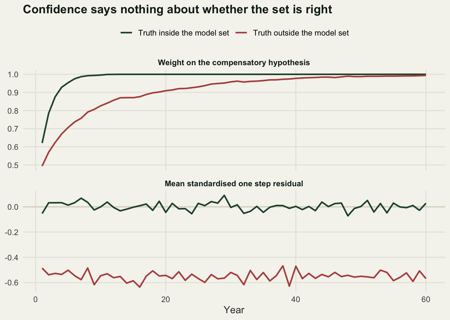
Where to go next
The active rule used here prices exactly one round of learning and then stops. The full problem is a dynamic program over the belief state, solved backwards on a discretised weight, which is heavier machinery for the same qualitative answer at a larger magnitude. Before reaching for it, check whether the decision is sensitive to the uncertainty at all: if the same regulation is best under both hypotheses then learning is worth nothing and the whole apparatus is decoration. The expected value of information is the measurement that settles that, and it takes a few lines.
References
Walters CJ 1986 Adaptive Management of Renewable Resources. Macmillan, ISBN 978-0-02-947970-4
Williams BK 2011 Journal of Environmental Management 92(5):1346-1353 (10.1016/j.jenvman.2010.10.041)
Johnson FA, Moore CT, Kendall WL, Dubovsky JA, Caithamer DF, Kelley JR, Williams BK 1997 Journal of Wildlife Management 61(1):202-216 (10.2307/3802429)
Runge MC 2011 Journal of Fish and Wildlife Management 2(2):220-233 (10.3996/082011-JFWM-045)