library(ggplot2)

te_pal <- list(forest = "#275139", green = "#2f8f63", sage = "#93a87f",
               clay = "#b5534e", gold = "#cda23f", line = "#dad9ca",
               ink = "#16241d", paper = "#f5f4ee")

theme_te <- function() {
  theme_minimal(base_size = 12) +
    theme(panel.grid.minor = element_blank(),
          panel.grid.major = element_line(colour = "#e7e6dc"),
          plot.background = element_rect(fill = "#f5f4ee", colour = NA),
          panel.background = element_rect(fill = "#f5f4ee", colour = NA),
          plot.title = element_text(face = "bold", colour = te_pal$ink),
          axis.title = element_text(colour = "#2c3a31"))
}Structured decision making in R
R
conservation
decision analysis
ecology tutorial
ggplot2
Build a conservation consequence table in R, screen out dominated options, and measure how much of the final ranking is ecology and how much is bookkeeping.
A reserve manager has a declining wader population, a fixed budget, a public with opinions about where it may walk, and seven options on the table, one of which is to carry on as she is. Someone will eventually write a table with the options down the side and the objectives across the top, fill it in, and add up. That table is a consequence table, and building one is the part of structured decision making that everybody agrees on. What happens next is where the trouble lives.
Between the table and the recommendation sit three pieces of bookkeeping that are usually done in a single afternoon and almost never written down: the rule that puts objectives on different scales onto a common one, the weights, and the set of alternatives that made it into the table at all. This tutorial builds a small decision from an explicit population and cost model, then measures how much of the resulting ranking comes from the ecology and how much from those three choices. All three can move the winner here, and one of them can be moved by an option that everyone in the room has already agreed to reject.
The costing side is treated separately in conservation costs and return on investment, which does the single-objective version: one currency, one ranking, no weights needed. Everything here starts where that ends, at the point where you have more than one thing you care about and no exchange rate between them that anyone will sign.
A reserve, seven options and four objectives
The site is a block of wet grassland holding 118 breeding pairs at the start of the decision, and the population has been shrinking. Five management actions are available. Scrub clearance with follow-up grazing restores open nesting habitat. Nest protection cages plus a warden reduce direct losses. Raising and holding water levels with new sluices improves chick food and buffers dry springs, which does more than any other action to lower year to year variability rather than simply raise the average. A predator exclusion fence around the core is the expensive option. A seasonal footpath closure removes disturbance during the nesting period.
Each action carries five numbers: an effect on the population growth rate if it is done alone, an effect on the environmental standard deviation, a capital cost, an annual cost, and a loss of public access in visitor days. Everything in the consequence table is computed from those.
n_years    <- 10
n0         <- 118
q_thresh   <- 60
r_base     <- -0.045
sd_base    <- 0.19
cap_pairs  <- 400
budget_cap <- 1600
visitor_base <- 42
disc        <- 0.035
annuity     <- (1 - (1 + disc)^(-n_years)) / disc
base_annual <- 8
dr_ceiling  <- 0.13
dsd_floor   <- 0.09
log_drop    <- log(n0 / q_thresh)

round(c(years = n_years, start_pairs = n0, quasi_extinction_at = q_thresh,
        baseline_growth = r_base, baseline_sd = sd_base,
        discount_rate = disc, annuity_factor = annuity,
        baseline_annual_cost = base_annual, visitor_days = visitor_base,
        growth_ceiling = dr_ceiling, sd_floor = dsd_floor,
        log_drop_to_threshold = log_drop,
        bound_pairs = cap_pairs, bound_cost = budget_cap), 4)
years start_pairs quasi_extinction_at
10.0000 118.0000 60.0000
baseline_growth baseline_sd discount_rate
-0.0450 0.1900 0.0350
annuity_factor baseline_annual_cost visitor_days
8.3166 8.0000 42.0000
growth_ceiling sd_floor log_drop_to_threshold
0.1300 0.0900 0.6763
bound_pairs bound_cost
400.0000 1600.0000 act <- data.frame(
name = c("scrub", "cages", "water", "fence", "closure", "summer scrub"),
dr = c(0.034, 0.026, 0.038, 0.052, 0.016, -0.060),
dsd = c(0, 0, -0.055, -0.005, 0, 0),
capital = c(95, 12, 240, 520, 4, 95),
annual = c(14, 32, 22, 26, 6, 14),
access = c(1, 3, 5, 8, 10, 4),
stringsAsFactors = FALSE)
n_act <- nrow(act)
print(act) name dr dsd capital annual access
1 scrub 0.034 0.000 95 14 1
2 cages 0.026 0.000 12 32 3
3 water 0.038 -0.055 240 22 5
4 fence 0.052 -0.005 520 26 8
5 closure 0.016 0.000 4 6 10
6 summer scrub -0.060 0.000 95 14 4lat_dr <- function(d) -dr_ceiling * log1p(-d / dr_ceiling)
lat_dsd <- function(d) dsd_floor * log1p(d / dsd_floor)
alt_names <- c("Status quo", "Scrub clearance", "Nest protection", "Water levels",
"Predator fence", "Water and scrub", "Full package")
alt_sets <- list(integer(0), 1L, 2L, 3L, 4L, c(1L, 3L), c(1L, 3L, 4L, 5L))
mem <- t(sapply(alt_sets, function(s) as.numeric(seq_len(n_act) %in% s)))
rownames(mem) <- alt_names
mem_bad <- rbind(mem, "Summer scrub clearance" = as.numeric(seq_len(n_act) == 6L))
c(alternatives = length(alt_names), objectives = 4)alternatives objectives
7 4 The sixth action in that table is not part of the decision yet. It is scrub clearance carried out in the breeding season instead of the winter, and it appears much later, for a specific purpose.
Log abundance follows a Brownian motion with drift: the drift is the growth rate an alternative buys, and the diffusion is environmental variability. Actions combine on a latent scale and saturate, so the growth uplift can never exceed 0.13 and the reduction in the standard deviation can never exceed 0.09. A single action delivers exactly the uplift stated in the table above; a package delivers less than the sum, which is what the ceiling is for.
That model gives two of the four objectives in closed form. Expected pairs in year 10 is the mean of a lognormal, \(N_0 \exp(10r + 5\sigma^2)\). The probability that the population passes below the quasi-extinction threshold of 60 pairs at any point in the ten years is the first passage probability of Brownian motion to a barrier, which has a two term expression involving only the normal distribution function. Cost is the discounted ten year total, capital plus annual at a discount rate of 0.035, which gives an annuity factor of 8.3166. Access is visitor days retained out of a current 42 thousand a year. Two objectives are to be maximised, two minimised.
first_passage <- function(rr, ss) {
  sT <- ss * sqrt(n_years)
  t1 <- pnorm((-log_drop - rr * n_years) / sT)
  t2 <- exp(-2 * rr * log_drop / ss^2 +
              pnorm((-log_drop + rr * n_years) / sT, log.p = TRUE))
  out <- t1 + t2
  out[out > 1] <- 1
  out
}

consequences <- function(edr, edsd, cap, ann, acc, rb, sb, ba, M) {
  na <- nrow(M)
  rr <- dr_ceiling * (1 - exp(-(M %*% t(edr)) / dr_ceiling)) + rep(rb, each = na)
  ss <- -dsd_floor * (1 - exp((M %*% t(edsd)) / dsd_floor)) + rep(sb, each = na)
  list(pairs  = n0 * exp(n_years * rr + 0.5 * n_years * ss^2),
       cost   = t(cap %*% t(M)) + t(ann %*% t(M)) * annuity +
                  rep(ba * annuity, each = na),
       access = visitor_base - t(acc %*% t(M)),
       risk   = first_passage(rr, ss),
       rr = rr, ss = ss)
}

rep_rows <- function(v, nd) matrix(rep(v, each = nd), nd, length(v))

base_pars <- list(edr = lat_dr(act$dr), edsd = lat_dsd(act$dsd), cap = act$capital,
                  ann = act$annual, acc = act$access, rb = r_base, sb = sd_base)

table_of <- function(p, M) {
  z <- consequences(rep_rows(p$edr, 1), rep_rows(p$edsd, 1), rep_rows(p$cap, 1),
                    rep_rows(p$ann, 1), rep_rows(p$acc, 1), p$rb, p$sb, base_annual, M)
  tb <- cbind(pairs = z$pairs[, 1], cost = z$cost[, 1],
              access = z$access[, 1], risk = z$risk[, 1])
  rownames(tb) <- rownames(M)
  attr(tb, "growth") <- z$rr[, 1]; attr(tb, "sd") <- z$ss[, 1]
  tb
}

cons_tab <- table_of(base_pars, mem)
print(round(cbind(cons_tab, growth = attr(cons_tab, "growth"),
                  sd = attr(cons_tab, "sd")), 4))
pairs cost access risk growth sd
Status quo 90.1238 66.5328 42 0.5174 -0.0450 0.1900
Scrub clearance 126.6193 277.9653 41 0.3169 -0.0110 0.1900
Nest protection 116.8843 344.6642 39 0.3613 -0.0190 0.1900
Water levels 120.5193 489.4982 37 0.1454 -0.0070 0.1350
Predator fence 150.1763 802.7646 34 0.2148 0.0070 0.1850
Water and scrub 153.3043 700.9306 36 0.0569 0.0171 0.1350
Full package 210.9756 1491.0620 18 0.0104 0.0493 0.1331Doing nothing leaves 90.1 pairs after ten years and a 0.5174 chance of dropping below the threshold on the way, for 66.5 thousand pounds of continued baseline management and no loss of access. The full package leaves 211.0 pairs and a risk of 0.0104, costs 1491 thousand, and closes enough of the reserve to cut visitor days from 42 to 18 thousand a year. Between those two are five intermediate options, and no two of them agree about which end of the table is better.
Both closed forms deserve a check before anything is built on them. The simulator below steps log abundance forward in annual jumps and, for each jump, uses the Brownian bridge crossing probability rather than only looking at the endpoints, so it estimates the continuous time quantity the formula claims to give rather than a coarser annual census version of it.
sim_alt <- function(rr, ss, nrep) {
  x <- numeric(nrep); surv <- rep(1, nrep)
  for (tt in seq_len(n_years)) {
    y <- x + rr + ss * rnorm(nrep)
    pc <- exp(-2 * (x + log_drop) * (y + log_drop) / ss^2)
    pc[x <= -log_drop | y <= -log_drop] <- 1
    surv <- surv * (1 - pc)
    x <- y
  }
  c(pairs = mean(n0 * exp(x)), risk = 1 - mean(surv))
}

set.seed(20260720)
n_rep <- 20000
simmed <- t(sapply(seq_along(alt_names), function(i)
  sim_alt(attr(cons_tab, "growth")[i], attr(cons_tab, "sd")[i], n_rep)))
rownames(simmed) <- alt_names
print(round(cbind(simulated = simmed, closed_form = cons_tab[, c("pairs", "risk")]), 4))
pairs risk pairs risk
Status quo 90.1462 0.5168 90.1238 0.5174
Scrub clearance 127.2964 0.3175 126.6193 0.3169
Nest protection 117.5999 0.3578 116.8843 0.3613
Water levels 120.7244 0.1413 120.5193 0.1454
Predator fence 149.2890 0.2204 150.1763 0.2148
Water and scrub 153.2110 0.0562 153.3043 0.0569
Full package 210.5571 0.0109 210.9756 0.0104c(replicates = n_rep)replicates
20000 round(c(max_rel_error_pairs = max(abs(simmed[, "pairs"] / cons_tab[, "pairs"] - 1)),
max_abs_error_risk = max(abs(simmed[, "risk"] - cons_tab[, "risk"]))), 5)max_rel_error_pairs max_abs_error_risk
0.00612 0.00560 Across 20000 replicates the worst relative disagreement on expected pairs is 0.00612 and the worst absolute disagreement on quasi-extinction risk is 0.0056, both of which are sampling noise at this replicate count. The formulae are doing what they claim, which matters because the rest of the post evaluates the consequence table hundreds of thousands of times.
What can be settled before anyone argues about weights
The first thing to do with a consequence table is not to score it. An alternative is dominated if some other alternative is at least as good on every objective and strictly better on at least one. A dominated alternative can be removed from the table without anyone stating a single preference, because whatever your weights, the alternative that dominates it scores at least as well. This is the only step in the whole analysis that is free of value judgements, so it is worth doing carefully and worth doing first.
The vectorised implementation below compares each row against all rows at once. Vectorised dominance code is easy to get subtly wrong, usually by forgetting the strictness condition and thereby marking identical rows as dominating each other, so it is checked against a brute force double loop that follows the definition literally.
orient <- c(pairs = 1, cost = -1, access = 1, risk = -1)
benefit <- function(tab) tab * rep(orient[colnames(tab)], each = nrow(tab))

dominated_set <- function(tab) {
  b <- benefit(tab)
  sapply(seq_len(nrow(b)), function(i) {
    ge <- t(t(b) >= b[i, ]); gt <- t(t(b) > b[i, ])
    any(rowSums(ge) == ncol(b) & rowSums(gt) >= 1)
  })
}

dominated_brute <- function(tab) {
  b <- benefit(tab); n <- nrow(b); out <- logical(n)
  for (i in seq_len(n)) for (j in seq_len(n)) {
    if (i == j) next
    ok <- TRUE; strict <- FALSE
    for (k in seq_len(ncol(b))) {
      if (b[j, k] < b[i, k]) ok <- FALSE
      if (b[j, k] > b[i, k]) strict <- TRUE
    }
    if (ok && strict) out[i] <- TRUE
  }
  out
}

dm <- dominated_set(cons_tab)
print(data.frame(alternative = alt_names, dominated = dm,
                 brute_force = dominated_brute(cons_tab)))
alternative dominated brute_force
1 Status quo FALSE FALSE
2 Scrub clearance FALSE FALSE
3 Nest protection TRUE TRUE
4 Water levels FALSE FALSE
5 Predator fence TRUE TRUE
6 Water and scrub FALSE FALSE
7 Full package FALSE FALSEc(agree = identical(dm, dominated_brute(cons_tab)),
dominated = sum(dm), efficient = sum(!dm)) agree dominated efficient
1 2 5 The two implementations agree exactly. Two of the seven alternatives are dominated, leaving an efficient set of five. Nest protection is dominated by scrub clearance, which delivers more pairs (126.6 against 116.9), costs less (278.0 against 344.7 thousand), keeps more of the reserve open and carries lower risk. The predator fence is dominated by water levels combined with scrub clearance: 153.3 pairs against 150.2, 700.9 thousand against 802.8, more access, and a risk of 0.0569 against 0.2148. Capital-heavy and labour-heavy actions both struggle against cheaper habitat work once you look at ten years of discounted spending.
Water levels is the interesting survivor. It produces fewer pairs than scrub clearance (120.5 against 126.6) and costs more, so on three of the four objectives it is beaten outright. It stays in the efficient set on the strength of one number: it cuts quasi-extinction risk to 0.1454 against 0.3169, because it is the single action that does most to reduce environmental variability, not merely to lift the mean. That is a real ecological distinction and the screening step preserves it without needing to know how much anyone cares about it.
lo_b <- c(pairs = 0, cost = 0, access = 0, risk = 0)
hi_b <- c(pairs = cap_pairs, cost = budget_cap, access = visitor_base, risk = 1)
score_bounds <- function(tab) {
  out <- tab
  for (k in colnames(tab))
    out[, k] <- if (orient[k] > 0) (tab[, k] - lo_b[k]) / (hi_b[k] - lo_b[k]) else
      (hi_b[k] - tab[, k]) / (hi_b[k] - lo_b[k])
  out
}

obj_lab <- c("Breeding pairs\nin year 10", "Ten year cost\n(GBP thousand)",
             "Visitor days\n(thousand a year)", "Quasi-extinction\nrisk")
disp <- ifelse(dm, paste0(alt_names, " (dominated)"), alt_names)
cell_txt <- c(sprintf("%.0f", cons_tab[, "pairs"]), sprintf("%.0f", cons_tab[, "cost"]),
              sprintf("%.1f", cons_tab[, "access"]), sprintf("%.3f", cons_tab[, "risk"]))
hm <- data.frame(alt = factor(rep(disp, 4), levels = rev(disp)),
                 obj = factor(rep(obj_lab, each = length(alt_names)), levels = obj_lab),
                 score = as.vector(score_bounds(cons_tab)), lab = cell_txt)

ggplot(hm, aes(obj, alt, fill = score)) +
  geom_tile(colour = te_pal$paper, linewidth = 1.2) +
  geom_text(aes(label = lab, colour = score > 0.55), size = 3.5, show.legend = FALSE) +
  scale_fill_gradient(low = "#e8e6d8", high = te_pal$forest, name = "Score",
                      limits = c(0, 1)) +
  scale_colour_manual(values = c("TRUE" = te_pal$paper, "FALSE" = te_pal$ink)) +
  labs(x = NULL, y = NULL, title = "No alternative is best on everything") +
  theme_te() +
  theme(panel.grid.major = element_blank(), legend.position = "right")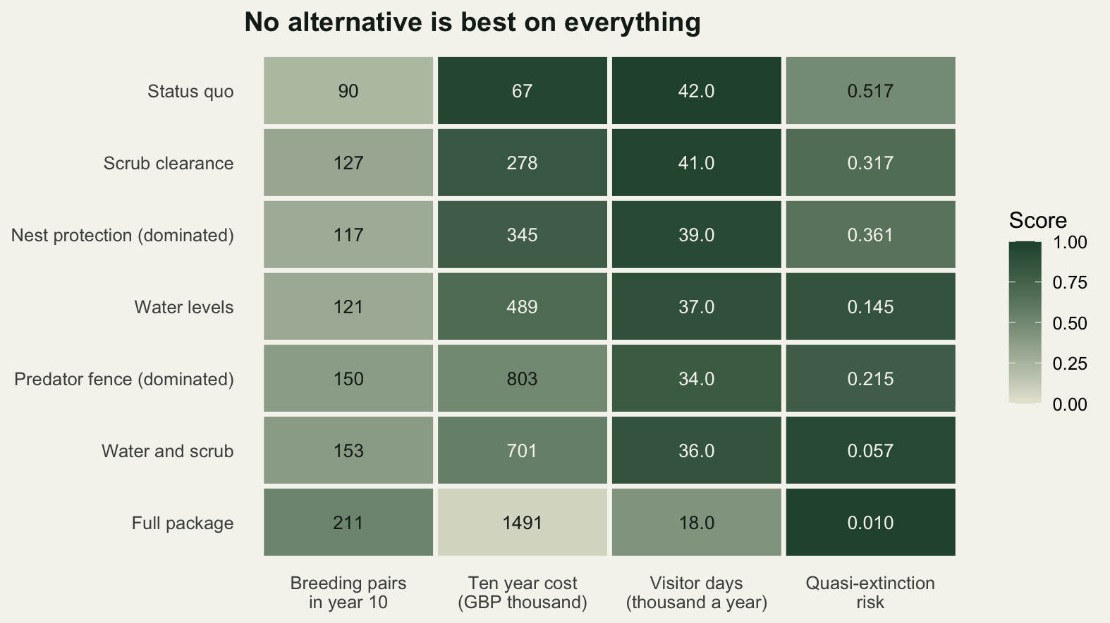
Three ways to make four objectives comparable
Five alternatives, four objectives, and no dominance left to exploit. To go further you must put pairs, pounds, visitor days and a probability on one scale. Three rules are in common use and all three look innocent.
Min-max scaling maps the worst alternative in the set to zero and the best to one, on each objective separately. Proportional scoring divides each value by the best value in the set, which for an objective to be minimised means dividing the smallest value by each value. Scaling against natural bounds ignores the alternatives entirely and uses externally stated limits: zero to 400 pairs, which is the reserve’s estimated habitat capacity, zero to 1600 thousand pounds, which is the trust’s ten year ceiling for this site, zero to the current 42 thousand visitor days, and zero to one for a probability.
Apply equal weights, which is what happens when nobody wants to argue about weights, and score the table three ways.
score_minmax <- function(tab) {
  b <- benefit(tab)
  out <- apply(b, 2, function(x) (x - min(x)) / (max(x) - min(x)))
  rownames(out) <- rownames(tab); out
}
score_prop <- function(tab) {
  out <- tab
  for (k in colnames(tab))
    out[, k] <- if (orient[k] > 0) tab[, k] / max(tab[, k]) else min(tab[, k]) / tab[, k]
  out
}

eqw <- c(pairs = 0.25, cost = 0.25, access = 0.25, risk = 0.25)
v_of <- function(s, w) as.vector(s %*% w[colnames(s)])

s_nb <- score_bounds(cons_tab)
val <- cbind(minmax = v_of(score_minmax(cons_tab), eqw),
             proportional = v_of(score_prop(cons_tab), eqw),
             natural_bounds = v_of(s_nb, eqw))
rownames(val) <- alt_names
print(round(val, 4))
minmax proportional natural_bounds
Status quo 0.5000 0.6118 0.6666
Scrub clearance 0.6269 0.4621 0.7005
Nest protection 0.5523 0.4261 0.6610
Water levels 0.6200 0.4149 0.6827
Predator fence 0.5609 0.4132 0.6171
Water and scrub 0.6839 0.4654 0.6864
Full package 0.5000 0.6183 0.5034rk <- apply(-val, 2, rank)
print(rk) minmax proportional natural_bounds
Status quo 6.5 2 4
Scrub clearance 2.0 4 1
Nest protection 5.0 5 5
Water levels 3.0 6 3
Predator fence 4.0 7 6
Water and scrub 1.0 3 2
Full package 6.5 1 7cat("top under each rule:", alt_names[apply(val, 2, which.max)], "\n")top under each rule: Water and scrub Full package Scrub clearance round(c(spearman_minmax_prop = cor(rk[, 1], rk[, 2], method = "spearman"),
spearman_minmax_bounds = cor(rk[, 1], rk[, 3], method = "spearman"),
spearman_prop_bounds = cor(rk[, 2], rk[, 3], method = "spearman"),
alternatives_changing_rank =
sum(apply(rk, 1, function(z) length(unique(z)) > 1))), 4) spearman_minmax_prop spearman_minmax_bounds
-0.3784 0.7748
spearman_prop_bounds alternatives_changing_rank
-0.0714 6.0000 val_eff <- cbind(minmax = v_of(score_minmax(cons_tab[!dm, ]), eqw),
proportional = v_of(score_prop(cons_tab[!dm, ]), eqw),
natural_bounds = v_of(score_bounds(cons_tab[!dm, ]), eqw))
c(max_change_after_dropping_dominated = max(abs(val_eff - val[!dm, ])))max_change_after_dropping_dominated
0 Three rules, three different winners. Min-max puts water and scrub on top with 0.6839. Proportional scoring puts the full package on top with 0.6183. Natural bounds put scrub clearance on top with 0.7005. Nothing about the reserve changed between those three lines; the ecology, the costs and the weights are identical.
The rank correlations show how little the three agree. Min-max and natural bounds correlate at 0.7748, which is the closest pair. Min-max and proportional correlate at -0.3784, and proportional against natural bounds at -0.0714, which is to say no relationship at all. Six of the seven alternatives sit at a different rank under at least one rule.
Two features of the min-max column are worth staring at. The status quo and the full package both score exactly 0.5000. That is not a fact about the reserve: under min-max each is best on two objectives and worst on the other two, so with equal weights each collects two ones and two zeros. The scale invented the tie. The proportional column has its own pathology at the other end. The full package scores 0.6183 largely because its quasi-extinction risk of 0.0104 is the smallest in the table, and dividing the smallest value by each value hands the winner a score of one and everybody else a small fraction. Ratio scoring on an objective whose best value is near zero is an amplifier.
One reassuring result before the bad news. Dropping the two dominated alternatives and rescoring the remaining five changes no score under any of the three rules: the largest absolute change is 0. That is what should happen, and it is worth measuring rather than assuming, because it sets up the contrast with the next section.
An option nobody would choose, changing the answer
A trustee asks a fair question at the meeting. The contractor who does the scrub clearance is only free in June. What if the work has to happen in the breeding season instead of the winter? The ecologist costs it: identical capital and identical annual spend, a net harm to productivity because the machinery is on the nesting fields, and more lost access because the works now fall in the visitor season. The option is added to the table.
It is immediately dismissed, and correctly. It costs exactly what winter scrub clearance costs and is worse on every other objective, so it is dominated. Nobody argues. But it is left in the table, because deleting rows from a table circulated to a board feels like hiding something.
tab2 <- table_of(base_pars, mem_bad)
print(round(tab2[, 1:4], 4))
pairs cost access risk
Status quo 90.1238 66.5328 42 0.5174
Scrub clearance 126.6193 277.9653 41 0.3169
Nest protection 116.8843 344.6642 39 0.3613
Water levels 120.5193 489.4982 37 0.1454
Predator fence 150.1763 802.7646 34 0.2148
Water and scrub 153.3043 700.9306 36 0.0569
Full package 210.9756 1491.0620 18 0.0104
Summer scrub clearance 49.4610 277.9653 38 0.8369print(data.frame(alternative = rownames(tab2), dominated = dominated_set(tab2),
brute_force = dominated_brute(tab2))) alternative dominated brute_force
1 Status quo FALSE FALSE
2 Scrub clearance FALSE FALSE
3 Nest protection TRUE TRUE
4 Water levels FALSE FALSE
5 Predator fence TRUE TRUE
6 Water and scrub FALSE FALSE
7 Full package FALSE FALSE
8 Summer scrub clearance TRUE TRUEval2 <- cbind(minmax = v_of(score_minmax(tab2), eqw),
proportional = v_of(score_prop(tab2), eqw),
natural_bounds = v_of(score_bounds(tab2), eqw))
rownames(val2) <- rownames(tab2)
print(round(val2, 4)) minmax proportional natural_bounds
Status quo 0.6596 0.6118 0.6666
Scrub clearance 0.7292 0.4621 0.7005
Nest protection 0.6682 0.4261 0.6610
Water levels 0.6929 0.4149 0.6827
Predator fence 0.6315 0.4132 0.6171
Water and scrub 0.7228 0.4654 0.6864
Full package 0.5000 0.6183 0.5034
Summer scrub clearance 0.4212 0.3478 0.5045keep <- seq_along(alt_names)
print(data.frame(alternative = alt_names,
minmax_before = rank(-val[, 1]), minmax_after = rank(-val2[keep, 1]))) alternative minmax_before minmax_after
Status quo Status quo 6.5 5
Scrub clearance Scrub clearance 2.0 1
Nest protection Nest protection 5.0 4
Water levels Water levels 3.0 3
Predator fence Predator fence 4.0 6
Water and scrub Water and scrub 1.0 2
Full package Full package 6.5 7cat("min-max winner before:", alt_names[which.max(val[, 1])],
"| after:", rownames(val2)[which.max(val2[, 1])], "\n")min-max winner before: Water and scrub | after: Scrub clearance round(c(minmax_max_score_change = max(abs(val2[keep, 1] - val[, 1])),
proportional_max_score_change = max(abs(val2[keep, 2] - val[, 2])),
bounds_max_score_change = max(abs(val2[keep, 3] - val[, 3])),
alternatives_changing_rank_minmax =
sum(rank(-val[, 1]) != rank(-val2[keep, 1]))), 5) minmax_max_score_change proportional_max_score_change
0.15957 0.00000
bounds_max_score_change alternatives_changing_rank_minmax
0.00000 6.00000 Summer scrub clearance leaves 49.5 pairs, costs the same 278.0 thousand as the winter version, retains 38 thousand visitor days and carries a quasi-extinction risk of 0.8369. It is dominated, it scores last, and no decision maker would ever pick it.
Under min-max scaling it changes the recommendation. The winner moves from water and scrub to scrub clearance. Six of the seven original alternatives change rank, and the largest change to a single alternative’s score is 0.15957, on a scale where the whole set of scores had run from 0.5000 to 0.6839. The status quo climbs from a shared sixth to fifth; the predator fence falls from fourth to sixth; the full package, previously tied on 0.5000, ends up alone in last.
Under proportional scoring and under natural bounds, the largest change to any score is 0. Not small: zero.
That contrast is the whole mechanism, and it is exact rather than empirical. Min-max scaling reads two numbers off the alternative set for each objective, the worst and the best. Summer scrub clearance is the worst in the table on breeding pairs and on risk, so it resets the bottom of both scales, and every other alternative’s score on those objectives is recomputed against a new denominator. Proportional scoring reads only the best value on each objective, and a dominated alternative can never be the best at anything, so proportional scores cannot move. Natural bounds read nothing from the set at all.
The general statement follows. Adding a dominated alternative changes a min-max ranking exactly when the new alternative sets a new extreme on some objective. The failure has a name in the decision analysis literature: it is a violation of independence of irrelevant alternatives, and the resulting reordering is rank reversal. It survives peer review, because a reviewer checks that the arithmetic is right and that the options are sensibly costed, and both are. Note also what the earlier measurement established: dominance screening does not protect you unless you delete the rows. Dropping the two dominated alternatives changed nothing, but that was because neither held an extreme. This one does.
alt_cols <- c("#cda23f", "#275139", "#93a87f", "#2f8f63", "#16241d", "#c9793f", "#b5534e")
names(alt_cols) <- alt_names
rule_lab <- c("Min-max\nwithin the set", "Proportional\nto the best",
              "Against natural\nbounds", "Min-max, with the\ndismissed option")
rank_tab <- cbind(rk, rank(-val2[keep, 1]))
bump <- data.frame(alt = factor(rep(alt_names, 4), levels = alt_names),
                   rule = factor(rep(rule_lab, each = length(alt_names)),
                                 levels = rule_lab),
                   rnk = as.vector(rank_tab))

ggplot(bump, aes(rule, rnk, colour = alt, group = alt)) +
  geom_line(linewidth = 0.9) +
  geom_point(size = 2.6) +
  scale_y_reverse(breaks = 1:7) +
  scale_colour_manual(values = alt_cols, name = NULL) +
  labs(x = NULL, y = "Rank under equal weights",
       title = "Four bookkeeping rules, four rankings") +
  theme_te() +
  theme(legend.position = "right")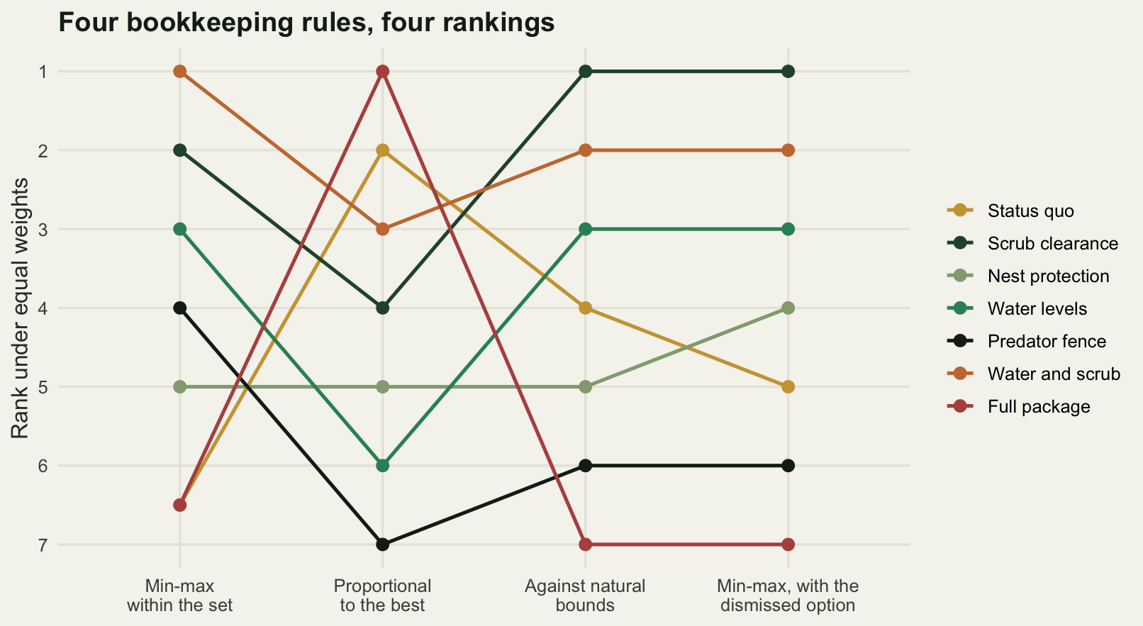
Natural bounds are the rule to use, and the rest of this post uses them. They are not free of judgement, since somebody chose 400 pairs and 1600 thousand pounds, but the judgement is stated once, in the open, and does not move when the option set changes.
Weights that know how much is at stake
Equal weights are not neutral. Read as a statement about swings, setting all four weights to 0.25 says that moving from the worst option in the table to the best on visitor access is worth exactly as much as moving from the cheapest option to the dearest. In this table the first swing is 24 thousand visitor days a year and the second is 1424.5 thousand pounds. Whatever the manager believes, she almost certainly does not believe those are equal.
Swing weighting fixes this by construction. The weight on an objective is not a statement about how important the objective sounds; it is a statement about how much the swing from the worst to the best level in this table is worth. Elicit an exchange rate per natural unit, multiply by the range the objective actually takes across the alternatives, and normalise. Here the manager states that one additional breeding pair in year 10 is worth 6 thousand pounds to the trust, that a thousand visitor days a year is worth 25 thousand pounds over the decade, and that one percentage point of quasi-extinction risk is worth 14 thousand pounds, which is 1400 thousand for the whole zero to one range. Cost is its own numeraire.
val_rate <- c(pairs = 6, cost = 1, access = 25, risk = 1400)
swing_weights <- function(tab, rates = val_rate) {
  rng <- apply(tab[, names(orient)], 2, function(x) diff(range(x)))
  w <- rng * rates[names(rng)]
  w / sum(w)
}
sw <- swing_weights(cons_tab)
print(round(rbind(range = apply(cons_tab, 2, function(x) diff(range(x))),
                  value_per_unit = val_rate,
                  swing_value = apply(cons_tab, 2, function(x) diff(range(x))) * val_rate,
                  swing_weight = sw, equal_weight = eqw), 4))
pairs cost access risk
range 120.8518 1424.5292 24.0000 0.5070
value_per_unit 6.0000 1.0000 25.0000 1400.0000
swing_value 725.1109 1424.5292 600.0000 709.8206
swing_weight 0.2096 0.4118 0.1734 0.2052
equal_weight 0.2500 0.2500 0.2500 0.2500v_eq <- v_of(s_nb, eqw); v_sw <- v_of(s_nb, sw)
names(v_eq) <- names(v_sw) <- alt_names
print(round(rbind(equal = v_eq, swing = v_sw), 4)) Status quo Scrub clearance Nest protection Water levels Predator fence
equal 0.6666 0.7005 0.6610 0.6827 0.6171
swing 0.7143 0.7161 0.6764 0.6771 0.5854
Water and scrub Full package
equal 0.6864 0.5034
swing 0.6539 0.4160cat("winner under equal weights:", alt_names[which.max(v_eq)],
"| under swing weights:", alt_names[which.max(v_sw)], "\n")winner under equal weights: Scrub clearance | under swing weights: Scrub clearance margin_of <- function(v) as.numeric(-diff(sort(v, decreasing = TRUE)[1:2]))
round(c(equal_margin = margin_of(v_eq), swing_margin = margin_of(v_sw)), 5)equal_margin swing_margin
0.01418 0.00173 print(round(rbind(all_seven = sw, efficient_five = swing_weights(cons_tab[!dm, ]),
with_dismissed_option = swing_weights(tab2)), 4)) pairs cost access risk
all_seven 0.2096 0.4118 0.1734 0.2052
efficient_five 0.2096 0.4118 0.1734 0.2052
with_dismissed_option 0.2335 0.3432 0.1446 0.2788The four swings are worth 725.1, 1424.5, 600 and 709.8 thousand pounds, giving weights of 0.2096 on pairs, 0.4118 on cost, 0.1734 on access and 0.2052 on risk. Cost gets about two thirds more weight than equal weighting gave it, and access loses roughly a third of its weight, because the range of access across these seven options is narrow in value terms.
The winner does not change. Scrub clearance tops both lists, which was not what I expected from a weight change of that size, and what happened underneath is more informative than a winner swap would have been. The margin collapsed: under equal weights scrub clearance led by 0.01418, under swing weights by 0.00173, a tenth as much. The runner-up changed identity, water and scrub falling from second to fifth and the status quo rising from fourth to second. A report quoting only the winner would have shown no change at all while the recommendation became a coin toss.
Swing weights inherit one weakness from the scaling rules, and it is the same weakness. They depend on the ranges, and the ranges depend on which alternatives are in the table. Here the weights computed on all seven alternatives and on the efficient five are identical to four decimal places, because the status quo and the full package hold the extremes on every objective and both are efficient. Recompute them with the dismissed summer option in the table and they move to 0.2335, 0.3432, 0.1446 and 0.2788. The rejected option that cannot be chosen has changed the weights by more than the difference between two reasonable analysts.
How far a weight has to move
A recommendation that survives the weights it was given is not the same as a recommendation that survives the weights it might have been given. The honest measure is a distance: how far does one weight have to move before the top two alternatives swap, with the other three rescaled so the weights still sum to one?
Because the value function is linear in the weights, this has a closed form. Write \(d_j\) for the difference in scores between the top two alternatives on objective \(j\), and let that objective’s weight move by \(\delta\) while the others are multiplied by \((1 - w_j - \delta)/(1 - w_j)\). The value difference is linear in \(\delta\), so the crossing point solves in one line, and the solution is substituted back and checked against zero.
ord <- order(-v_sw)
a1 <- ord[1]; a2 <- ord[2]
dsc <- s_nb[a1, ] - s_nb[a2, ]

flip_delta <- function(j) {
  dj <- dsc[j]; wj <- sw[j]; rest <- sum(dsc[-j] * sw[-j])
  den <- dj - rest / (1 - wj)
  if (abs(den) < 1e-12) return(NA_real_)
  d <- -(dj * wj + rest) / den
  if (d < -wj || d > 1 - wj) return(NA_real_)
  d
}
fl <- sapply(seq_along(sw), flip_delta); names(fl) <- names(sw)

recheck <- sapply(seq_along(sw), function(j) {
  if (is.na(fl[j])) return(NA_real_)
  w <- sw; w[j] <- sw[j] + fl[j]; w[-j] <- sw[-j] * (1 - w[j]) / (1 - sw[j])
  sum(dsc * w)
})

cat("top two under swing weights:", alt_names[a1], "and", alt_names[a2], "\n")
top two under swing weights: Scrub clearance and Status quo print(round(rbind(score_difference = dsc, swing_weight = sw,
weight_at_flip = sw + fl, move_needed = fl), 4)) pairs cost access risk
score_difference 0.0912 -0.1321 -0.0238 0.2006
swing_weight 0.2096 0.4118 0.1734 0.2052
weight_at_flip 0.1943 0.4194 0.2295 0.1983
move_needed -0.0153 0.0076 0.0560 -0.0069round(c(value_gap = v_sw[a1] - v_sw[a2],
smallest_move = min(abs(fl), na.rm = TRUE),
max_recheck_residual = max(abs(recheck), na.rm = TRUE)), 6)value_gap.Scrub clearance smallest_move max_recheck_residual
0.001732 0.006922 0.000000 The substitution check returns a maximum residual of 0, so the algebra is right. The top two are scrub clearance and the status quo, separated by 0.001732 of value. Every one of the four weights can flip that ordering on its own, and the directions are the ones the score differences imply. Lowering the weight on quasi-extinction risk from 0.2052 to 0.1983, a move of 0.0069, is the cheapest flip. Raising the weight on cost by 0.0076 does it, as does lowering the weight on breeding pairs by 0.0153 or raising the weight on visitor access by 0.0560.
The smallest move across all four objectives is 0.006922, and that is the number to report next to the recommendation. It says that the analysis prefers scrub clearance to doing nothing by a margin that a change of seven parts in a thousand in one weight erases. No amount of care over the population model would improve that, because the model is not what is close.
obj_short <- c(pairs = "Breeding pairs", cost = "Ten year cost",
               access = "Visitor access", risk = "Quasi-extinction risk")
sens <- data.frame(obj = factor(obj_short[names(sw)], levels = rev(obj_short)),
                   w0 = as.numeric(sw), w1 = as.numeric(sw + fl))

ggplot(sens, aes(y = obj)) +
  geom_vline(xintercept = 0.25, colour = te_pal$line, linewidth = 0.9) +
  geom_segment(aes(x = w0, xend = w1, yend = obj), colour = te_pal$sage,
               linewidth = 3.4, lineend = "butt") +
  geom_point(aes(x = w0), colour = te_pal$forest, size = 3) +
  geom_point(aes(x = w1), colour = te_pal$clay, size = 3, shape = 18) +
  annotate("text", x = 0.255, y = 0.62, label = "equal weights", hjust = 0,
           size = 3, colour = "#2c3a31") +
  scale_x_continuous(limits = c(0, 0.5)) +
  labs(x = "Weight on the objective", y = NULL,
       title = "The recommendation does not survive a small change in one weight",
       subtitle = "Circle: elicited swing weight. Diamond: the weight at which the top two swap.") +
  theme_te() +
  theme(plot.subtitle = element_text(colour = "#2c3a31", size = 9))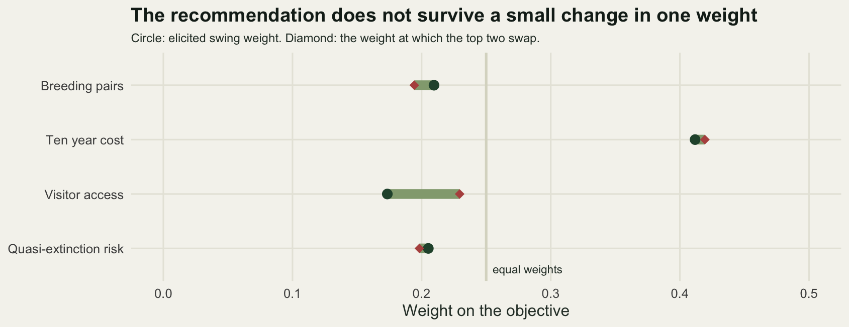
The probability of being best
Every number in the consequence table is an estimate. The effect of scrub clearance on the growth rate is not known to three decimals; capital costs overrun; the response of visitors to a closed path is a guess. Put a distribution on the inputs, push it through the same model, and ask a different question of the table: not which alternative has the highest expected score, but how often each alternative comes out on top.
cv_dr <- 0.35; cv_dsd <- 0.30; cv_cap <- 0.25; cv_ann <- 0.15; cv_acc <- 0.30
sd_rbase <- 0.012; cv_sdbase <- 0.15
round(c(cv_growth_effect = cv_dr, cv_variance_effect = cv_dsd, cv_capital = cv_cap,
        cv_annual = cv_ann, cv_access = cv_acc, sd_baseline_growth = sd_rbase,
        cv_baseline_sd = cv_sdbase), 4)
cv_growth_effect cv_variance_effect cv_capital cv_annual
0.350 0.300 0.250 0.150
cv_access sd_baseline_growth cv_baseline_sd
0.300 0.012 0.150 ln_mult <- function(cv, n) { s <- sqrt(log(1 + cv^2)); exp(rnorm(n, -s^2 / 2, s)) }
draw_pars <- function(nd, p = base_pars) {
list(edr = rep_rows(p$edr, nd) * matrix(ln_mult(cv_dr, nd * n_act), nd, n_act),
edsd = rep_rows(p$edsd, nd) * matrix(ln_mult(cv_dsd, nd * n_act), nd, n_act),
cap = rep_rows(p$cap, nd) * matrix(ln_mult(cv_cap, nd * n_act), nd, n_act),
ann = rep_rows(p$ann, nd) * matrix(ln_mult(cv_ann, nd * n_act), nd, n_act),
acc = rep_rows(p$acc, nd) * matrix(ln_mult(cv_acc, nd * n_act), nd, n_act),
rb = rnorm(nd, p$rb, sd_rbase),
sb = p$sb * ln_mult(cv_sdbase, nd),
ba = rep(base_annual, nd))
}
score_draws <- function(z, w) {
(z$pairs / cap_pairs) * w["pairs"] +
((budget_cap - z$cost) / budget_cap) * w["cost"] +
(z$access / visitor_base) * w["access"] +
(1 - z$risk) * w["risk"]
}
set.seed(11)
n_draw <- 5000
pp <- draw_pars(n_draw)
zz <- consequences(pp$edr, pp$edsd, pp$cap, pp$ann, pp$acc, pp$rb, pp$sb, pp$ba, mem)
p_best <- tabulate(max.col(t(score_draws(zz, sw)), ties.method = "first"),
length(alt_names)) / n_draw
names(p_best) <- alt_names
c(draws = n_draw)draws
5000 print(round(rbind(point_value = v_sw, prob_best = p_best), 4)) Status quo Scrub clearance Nest protection Water levels
point_value 0.7143 0.7161 0.6764 0.6771
prob_best 0.4820 0.4684 0.0146 0.0346
Predator fence Water and scrub Full package
point_value 0.5854 0.6539 0.416
prob_best 0.0004 0.0000 0.000cat("point winner:", alt_names[which.max(v_sw)],
"| most likely best:", alt_names[which.max(p_best)], "\n")point winner: Scrub clearance | most likely best: Status quo c(draws_where_fence_beats_water_and_scrub_on_all_four =
sum(zz$pairs[5, ] > zz$pairs[6, ] & zz$cost[5, ] < zz$cost[6, ] &
zz$access[5, ] > zz$access[6, ] & zz$risk[5, ] < zz$risk[6, ]))draws_where_fence_beats_water_and_scrub_on_all_four
2 Over 5000 draws the status quo is best in 0.4820 of them and scrub clearance in 0.4684. The alternative that wins on the point estimate table is not the one most likely to be best. Nothing is wrong with either calculation. The point estimate table asks which alternative scores highest at the mean of the inputs; the probability of being best asks how often it comes first, and those are different questions whenever the two leaders are close and the uncertainty is asymmetric. Scrub clearance carries cost overrun risk and effect size risk that the status quo does not, so its score has a longer left tail, and a long left tail costs draws without costing much mean.
Water levels takes 0.0346 of the draws and nest protection 0.0146, both more than their point estimate ranks suggest. Nest protection is a dominated alternative that wins outright in one draw in seventy, which is a reminder about what the screening step established. Dominance was tested on the point estimate table. In 2 of the 5000 draws the predator fence beats water and scrub on all four objectives at once, so even the free step of the analysis is conditional on the numbers being right.
How often does the point estimate winner disagree with the most likely best? Once is an anecdote. The block below builds 200 different decision problems by perturbing the whole parameter set, including the manager’s exchange rates, and runs the full analysis on each: a point estimate table, swing weights computed from that table’s own ranges, then 800 draws to get the probability of being best.
jitter_pars <- function(p, f) {
  p$edr <- p$edr * ln_mult(f * cv_dr, n_act)
  p$edsd <- p$edsd * ln_mult(f * cv_dsd, n_act)
  p$cap <- p$cap * ln_mult(f * cv_cap, n_act)
  p$ann <- p$ann * ln_mult(f * cv_ann, n_act)
  p$acc <- p$acc * ln_mult(f * cv_acc, n_act)
  p$rb <- rnorm(1, p$rb, f * sd_rbase)
  p$sb <- p$sb * ln_mult(f * cv_sdbase, 1)
  p
}

set.seed(707)
n_inst <- 200; nd_inst <- 800
spread_factor <- 1.5; rate_cv <- 0.4
c(problems = n_inst, draws_each = nd_inst,
  between_problem_spread = spread_factor, exchange_rate_cv = rate_cv)
problems draws_each between_problem_spread
200.0 800.0 1.5
exchange_rate_cv
0.4 inst <- t(sapply(seq_len(n_inst), function(i) {
bs <- jitter_pars(base_pars, spread_factor)
tb <- table_of(bs, mem)
rates <- val_rate * c(ln_mult(rate_cv, 1), 1, ln_mult(rate_cv, 1), ln_mult(rate_cv, 1))
wi <- swing_weights(tb, rates)
vv <- v_of(score_bounds(tb), wi)
qq <- draw_pars(nd_inst, bs)
z2 <- consequences(qq$edr, qq$edsd, qq$cap, qq$ann, qq$acc, qq$rb, qq$sb, qq$ba, mem)
pb <- tabulate(max.col(t(score_draws(z2, wi)), ties.method = "first"),
length(alt_names)) / nd_inst
pw <- which.max(vv)
c(point = pw, likely = which.max(pb), p_point = pb[pw], p_max = max(pb),
gap = -diff(sort(vv, decreasing = TRUE)[1:2]))
}))
mismatch <- inst[, "point"] != inst[, "likely"]
tight <- inst[, "gap"] <= quantile(inst[, "gap"], 0.25)
round(c(mismatches = sum(mismatch), mismatch_rate = mean(mismatch),
tightest_quartile_gap_below = as.numeric(quantile(inst[, "gap"], 0.25)),
mismatch_rate_tightest_quartile = mean(mismatch[tight])), 4) mismatches mismatch_rate
7.0000 0.0350
tightest_quartile_gap_below mismatch_rate_tightest_quartile
0.0102 0.1400 ex <- which(mismatch)[order(-(inst[mismatch, "p_max"] - inst[mismatch, "p_point"]))[1]]
cat("example problem: point winner", alt_names[inst[ex, "point"]],
"with p(best) =", round(inst[ex, "p_point"], 4),
"| most likely best", alt_names[inst[ex, "likely"]],
"with p(best) =", round(inst[ex, "p_max"], 4), "\n")example problem: point winner Scrub clearance with p(best) = 0.4425 | most likely best Status quo with p(best) = 0.5438 round(c(example_point_value_gap = inst[ex, "gap"]), 5)example_point_value_gap.gap
0.00024 Across 200 problems the point estimate winner differed from the most likely best in 7 of them, a rate of 0.035. That is lower than the fuss around this distinction would lead you to expect, and it is the measurement, so it stands. The conditional version is the useful one. Split the problems by the value gap between the top two alternatives on the point estimate table and take the tightest quartile, where that gap is below 0.0102: the mismatch rate there is 0.14, higher than the overall rate. In the clearest example the point estimate winner, scrub clearance, is best in 0.4425 of draws while the status quo is best in 0.5438, and the two were separated on the point estimate table by 0.00024 of value.
The practical rule falls out of that. Computing the probability of being best is worth the effort when the top two are close and is decoration when they are not, and you already know which case you are in from the value gap, which costs nothing.
What the analysis cannot supply
The weights are value judgements. No amount of population modelling produces the exchange rate between a breeding pair and a thousand pounds, and any analysis that appears to produce one has smuggled it in. That is not a failure of structured decision making; it is the point of it, which is to separate the parts that can be measured from the parts that must be chosen. But it does raise the obvious question: if the weights are not knowable, what is the analysis for?
There is a measurement that answers it. Draw weight vectors uniformly from the simplex, meaning every combination of four non-negative weights summing to one is equally likely, and record which alternative comes top in each. If one alternative wins nearly everywhere, the weights barely matter and the analysis can say so out loud. If the winner is split, the weights are the decision, and the analysis has done its real job, which is to find out what the argument is actually about.
Both cases are constructed below. The first is the reserve as costed. The second is the same reserve after a national funder offers to meet the capital cost of whatever is chosen, to cover 85 per cent of the running costs, and to require the works outside the breeding and visitor seasons, which removes nine tenths of the access loss.
set.seed(99)
n_w <- 40000
wdraw <- matrix(rexp(n_w * 4), n_w, 4)
wdraw <- wdraw / rowSums(wdraw)
colnames(wdraw) <- names(eqw)

frac_win <- function(tab) {
  out <- tabulate(max.col(score_bounds(tab) %*% t(wdraw) |> t(), ties.method = "first"),
                  nrow(tab)) / n_w
  names(out) <- rownames(tab); out
}

grant_annual <- 0.15; grant_access <- 0.10
pars_f <- base_pars
pars_f$cap <- rep(0, n_act)
pars_f$ann <- act$annual * grant_annual
pars_f$acc <- act$access * grant_access
tab_f <- table_of(pars_f, mem)
print(round(tab_f[, 1:4], 3))
pairs cost access risk
Status quo 90.124 66.533 42.0 0.517
Scrub clearance 126.619 83.998 41.9 0.317
Nest protection 116.884 106.453 41.7 0.361
Water levels 120.519 93.978 41.5 0.145
Predator fence 150.176 98.968 41.2 0.215
Water and scrub 153.304 111.443 41.4 0.057
Full package 210.976 151.362 39.6 0.010c(weight_vectors = n_w)weight_vectors
40000 round(c(grant_share_of_running_cost_percent = 100 * (1 - grant_annual),
grant_share_of_access_loss_percent = 100 * (1 - grant_access),
running_cost_left = grant_annual, access_loss_left = grant_access), 2)grant_share_of_running_cost_percent grant_share_of_access_loss_percent
85.00 90.00
running_cost_left access_loss_left
0.15 0.10 print(round(rbind(as_costed = frac_win(cons_tab), if_funded = frac_win(tab_f)), 4)) Status quo Scrub clearance Nest protection Water levels
as_costed 0.2830 0.2765 0 0.0190
if_funded 0.0072 0.0161 0 0.0042
Predator fence Water and scrub Full package
as_costed 0.0000 0.3432 0.0785
if_funded 0.0013 0.1615 0.8097As costed, the largest share any alternative takes is 0.3432, which goes to water and scrub. The status quo takes 0.2830, scrub clearance 0.2765, the full package 0.0785 and water levels 0.0190. The weights are the decision. Anyone who reports a single recommended option from this table without that number beside it is reporting their own weights and calling it an analysis. What the analysis has bought is the shape of the disagreement: it is not about the population model, and it is not about which action works. It is about the exchange rate between money and birds, and about how much public access the trust is willing to trade for either.
Change the funding and the picture inverts. With capital paid and running costs cut to 0.15 of their level, the ten year cost of the full package falls from 1491 to 151.4 thousand, and the whole cost column collapses into a narrow band. The full package then wins 0.8097 of the simplex, water and scrub 0.1615 and everything else the remainder. On that version of the problem an analyst can tell the board something genuinely useful: the choice does not depend on how you weight these four objectives, so stop arguing about the weights and do the full package. The same population model, the same five actions, and a completely different kind of answer.
gstep <- 64
gg <- expand.grid(i = 0:gstep, j = 0:gstep)
gg <- gg[gg$i + gg$j <= gstep, ]
bary <- cbind(pairs = gg$i / gstep, cost = gg$j / gstep,
              access = 1 - (gg$i + gg$j) / gstep)
wgrid <- cbind(bary * (1 - sw["risk"]), risk = sw["risk"])
tri_xy <- function(b) data.frame(x = b[, "cost"] + 0.5 * b[, "access"],
                                 y = b[, "access"] * sqrt(3) / 2)

panel_lab <- c("As costed", "If a funder pays for the works")
map_df <- do.call(rbind, lapply(seq_along(panel_lab), function(k) {
  tb <- list(cons_tab, tab_f)[[k]]
  w <- max.col(t(score_bounds(tb) %*% t(wgrid)), ties.method = "first")
  data.frame(tri_xy(bary), alt = factor(alt_names[w], levels = alt_names),
             panel = panel_lab[k])
}))
map_df$panel <- factor(map_df$panel, levels = panel_lab)
sw_pt <- tri_xy(rbind(as.numeric(sw[c("pairs", "cost", "access")]) / (1 - sw["risk"])) |>
                  `colnames<-`(c("pairs", "cost", "access")))
corners <- data.frame(x = c(0, 1, 0.5), y = c(0, 0, sqrt(3) / 2),
                      lab = c("all weight on\nbreeding pairs", "all weight\non cost",
                              "all weight on\nvisitor access"),
                      vj = c(1.5, 1.5, -0.4), hj = c(0.1, 0.9, 0.5))

ggplot(map_df, aes(x, y, colour = alt)) +
  geom_point(shape = 15, size = 1.35) +
  geom_point(data = sw_pt, aes(x, y), inherit.aes = FALSE, shape = 4,
             colour = te_pal$ink, size = 3.4, stroke = 1.3) +
  geom_text(data = corners, aes(x, y, label = lab, vjust = vj, hjust = hj),
            inherit.aes = FALSE, size = 2.9, colour = "#2c3a31") +
  facet_wrap(~panel) +
  scale_colour_manual(values = alt_cols, name = NULL) +
  coord_equal(xlim = c(-0.16, 1.16), ylim = c(-0.15, 0.99)) +
  labs(x = NULL, y = NULL, title = "Where the weights decide, and where they do not") +
  theme_te() +
  theme(axis.text = element_blank(), panel.grid.major = element_blank(),
        strip.text = element_text(colour = te_pal$ink, face = "bold"))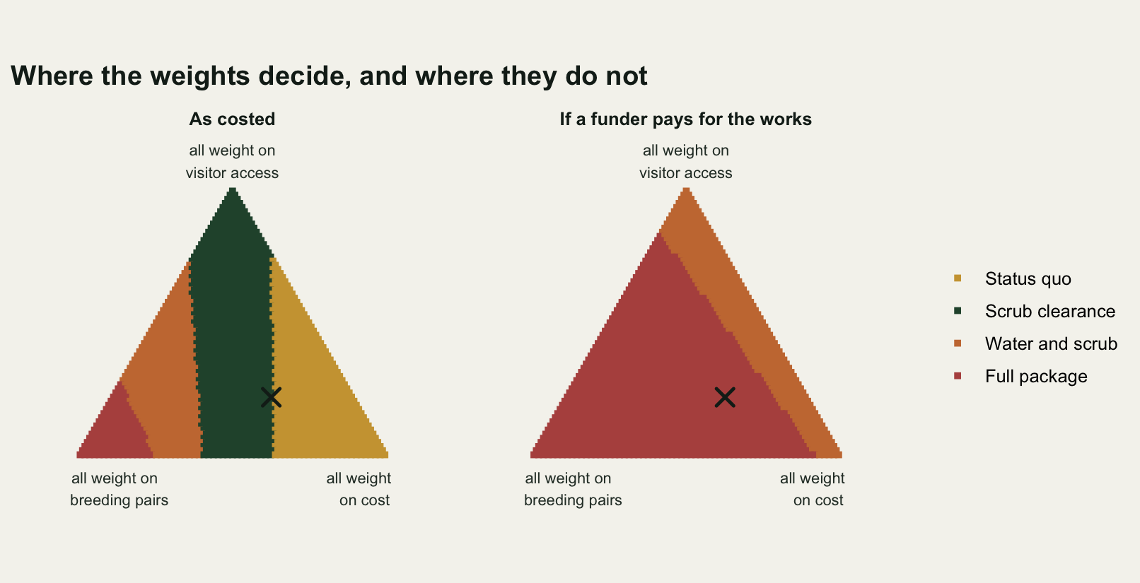
Three further limits deserve stating plainly, because the simplex measurement does not cover them. The additive value function assumes a pair is worth the same whether the population is at 90 or at 211, and that access and abundance do not interact; a value function with curvature can reorder the table on its own. The objectives are themselves a choice, and an objective that is not in the table has a weight of exactly zero whether anyone intended that or not. And the whole table rests on effect sizes for five actions that are known in the field to nothing like the precision used here, which is what the 0.35 coefficient of variation on the growth effects was standing in for.
Where to go next
The natural follow-up is to stop treating the consequence table as fixed. If the ranking hinges on an effect size nobody has measured, the question becomes whether it is worth buying that measurement before deciding, which is what the expected value of information puts a price on. Checking a decision analysis takes the other route and tries to break the machinery above with a set of deliberate stress tests, including the one this post did not run: what happens when the objectives themselves are correlated.
References
Gregory R, Failing L, Harstone M, Long G, McDaniels T, Ohlson D 2012 Structured Decision Making: A Practical Guide to Environmental Management Choices. Wiley-Blackwell, ISBN 978-1-4443-3341-1
Keeney RL, Raiffa H 1993 Decisions with Multiple Objectives: Preferences and Value Tradeoffs. Cambridge University Press, ISBN 978-0-521-44185-8
Martin J, Runge MC, Nichols JD, Lubow BC, Kendall WL 2009 Ecological Applications 19(5):1079-1090 (10.1890/08-0255.1)
Runge MC, Converse SJ, Lyons JE, Smith DR (eds) 2020 Structured Decision Making: Case Studies in Natural Resource Management. Johns Hopkins University Press, ISBN 978-1-4214-3756-9
Belton V, Gear T 1983 Omega 11(3):228-230 (10.1016/0305-0483(83)90047-6)