library(ggplot2)

te_pal <- list(forest = "#275139", green = "#2f8f63", sage = "#93a87f",
               clay = "#b5534e", gold = "#cda23f", line = "#dad9ca",
               ink = "#16241d", paper = "#f5f4ee")

theme_te <- function() {
  theme_minimal(base_size = 12) +
    theme(panel.grid.minor = element_blank(),
          panel.grid.major = element_line(colour = "#e7e6dc"),
          plot.background = element_rect(fill = "#f5f4ee", colour = NA),
          panel.background = element_rect(fill = "#f5f4ee", colour = NA),
          plot.title = element_text(face = "bold", colour = te_pal$ink),
          axis.title = element_text(colour = "#2c3a31"),
          axis.text = element_text(colour = "#2c3a31"),
          legend.position = "bottom")
}Eliciting probabilities from experts
R
decision analysis
Bayesian statistics
ecology tutorial
Simulate expert elicitation in R: the four-point question, overconfidence against nominal coverage, linear and logarithmic pooling, and Cooke weights.
A reintroduction programme has to state the probability that the founded population is still there in twenty years. There is no time series, because the population does not exist yet. There is no comparable release close enough to borrow from. The number goes into the business case anyway, and it comes from asking people who have worked with the species.
That is elicitation, and it is a procedure with a measurable output rather than a shrug. It has a literature, protocols with names, and failure modes that are known and repeatable. What matters about those failures is that they are not noise. They point in a direction: intervals come out too narrow, almost every time, from almost everybody, and the narrowness survives being pointed out.
This is a different job from the one an earlier post did. Structured decision making in R elicits weights: how much a unit of one objective is worth against a unit of another, taken from a single decision maker by a swing exchange rate. That is a value judgement, and there is no fact of the matter to check it against. Here the quantity is a belief about the world, so there is a right answer somewhere, the elicitation can be scored, and the quality control is entirely different. Weights get audited by sensitivity analysis; beliefs get audited by asking questions whose answers you already know.
Everything below runs on simulated experts. Each one has a genuine internal belief and a set of habits that damage it on the way out, and because the simulation knows both the truth and the belief, it can separate the two. That separation is the only reason any of this is measurable. Five things get measured: whether the question order changes the width of the answer, how far below nominal a stated 90 per cent interval actually falls, what changes when you combine experts by averaging densities rather than by multiplying them, whether performance weights earn their keep, and whether any of it reaches the decision the numbers were collected for.
An expert with a belief and a set of habits
The simulated expert has two layers. The inner layer is an honest belief about the quantity: a centre and a spread. The centre sits off the true value by an amount drawn from a normal with that same spread, which is the definition of being calibrated. If this expert could report the inner layer directly, their stated intervals would cover at exactly the nominal rate, forever.
The outer layer is what the questioning does to it. Two habits are modelled. The first is a standing bias: some people run optimistic about the species and some run pessimistic, and the offset is a property of the person, not the question. The second is anchoring and adjustment. Ask for a best guess and then for bounds, and the best guess becomes the anchor; the adjustment outward from it is systematically too small, by a factor that varies between people but is consistently below one.
The seed questions are quantities the expert does not know and the analyst does: a count from a survey that has not been published yet, a survival rate from a report in a drawer, the year a population last bred at a site. Values sit on a standardised scale so the units drop out. Twenty four experts, forty questions.
set.seed(20260730)
n_exp <- 24
n_item <- 40

s_int  <- exp(rnorm(n_exp, log(0.55), 0.35))
bias_e <- rnorm(n_exp, 0, 0.45)
phi_e  <- runif(n_exp, 0.35, 0.85)
psi_e  <- phi_e + runif(n_exp, 0.10, 0.35)
conf_e <- runif(n_exp, 0.70, 0.95)

theta <- rnorm(n_item, 0, 1)
mu_mat <- matrix(theta, n_exp, n_item, byrow = TRUE) + bias_e * s_int +
  matrix(rnorm(n_exp * n_item), n_exp) * s_int

zq <- function(q) qnorm(1 - (1 - q) / 2)
err <- abs(mu_mat - matrix(theta, n_exp, n_item, byrow = TRUE))
cover_at <- function(sg, q) rowMeans(err < zq(q) * sg)

print(round(c(experts = n_exp, questions = n_item,
              nominal_level_percent = 90,
              internal_sd_median = median(s_int),
              internal_sd_min = min(s_int), internal_sd_max = max(s_int),
              bias_sd_in_own_units = sd(bias_e),
              adjust_fraction_min = min(phi_e),
              adjust_fraction_max = max(phi_e)), 4))
experts questions nominal_level_percent
24.0000 40.0000 90.0000
internal_sd_median internal_sd_min internal_sd_max
0.5947 0.3008 1.1439
bias_sd_in_own_units adjust_fraction_min adjust_fraction_max
0.4159 0.4333 0.8279 print(round(c(honest_coverage_90 = mean(cover_at(s_int, 0.90)),
honest_coverage_50 = mean(cover_at(s_int, 0.50))), 4))honest_coverage_90 honest_coverage_50
0.9000 0.5042 If the inner belief were reported without damage, the coverage of a nominal 90 per cent interval across all 960 expert-question pairs would be 0.9, and of a nominal fifty per cent interval 0.5042. The biases are real and forty questions is a small sample, so the agreement is luckier than it looks, but it is close enough that everything below can be read as damage inflicted by the protocol rather than as a property of the people.
The four-point question against the direct one
The direct question is the one everybody asks first: give me a 90 per cent interval for this quantity. The expert forms a best guess, then widens outward by a fraction of the distance they should have gone, so the implied standard deviation of the reported interval is that fraction times their real one.
The four-point method of Speirs-Bridge and colleagues changes the order and adds a step. Ask for the realistically lowest value first, then the realistically highest, then the best guess, and then, last, ask how confident the expert is that the interval they just gave contains the truth. The first three questions remove the central anchor, because there is no best guess on the table when the bounds are set. The fourth turns the interval into something the analyst can rescale: if the expert puts their confidence in the bounds they drew below the level you asked for, then what they drew is a narrower interval than the one you wanted, and widening it to the level you wanted is a matter of the ratio of two normal quantiles.
Both steps are modelled here and both can be switched off, which is the point. The middle row of the table below is the four-point ordering with the confidence question thrown away, so the raw bounds are read as if they were a 90 per cent interval.
sig_direct <- phi_e * s_int
sig_bounds <- psi_e * s_int
sig_four   <- psi_e * zq(0.90) * s_int / zq(conf_e)

lv <- c(0.50, 0.60, 0.70, 0.80, 0.90, 0.95, 0.99)
cov_tab <- data.frame(
  nominal = lv,
  direct  = sapply(lv, function(q) mean(cover_at(sig_direct, q))),
  bounds  = sapply(lv, function(q) mean(cover_at(sig_bounds, q))),
  four    = sapply(lv, function(q) mean(cover_at(sig_four, q))))
print(round(cov_tab, 4))
nominal direct bounds four
1 0.50 0.3188 0.4281 0.4979
2 0.60 0.3917 0.5042 0.5865
3 0.70 0.4708 0.5990 0.7010
4 0.80 0.5448 0.7042 0.7781
5 0.90 0.6792 0.8104 0.8760
6 0.95 0.7562 0.8823 0.9302
7 0.99 0.8625 0.9552 0.9760rescale <- zq(0.90) / zq(conf_e)
print(round(c(width_ratio_four_over_direct = mean(sig_four / sig_direct),
fraction_of_experts_widened = mean(sig_four > sig_direct),
mean_rescale_factor = mean(rescale),
min_rescale_factor = min(rescale),
max_rescale_factor = max(rescale)), 4))width_ratio_four_over_direct fraction_of_experts_widened
1.7005 1.0000
mean_rescale_factor min_rescale_factor
1.2306 0.8556
max_rescale_factor
1.5763 c90d <- cover_at(sig_direct, 0.90)
c90b <- cover_at(sig_bounds, 0.90)
c90f <- cover_at(sig_four, 0.90)
print(round(c(gain_from_question_order = mean(c90b) - mean(c90d),
gain_from_rescaling = mean(c90f) - mean(c90b),
total_gain = mean(c90f) - mean(c90d)), 4))gain_from_question_order gain_from_rescaling total_gain
0.1312 0.0656 0.1969 The four-point intervals are wider than the direct ones for 100 per cent of the experts, by an average factor of 1.7005. The answer to the first question is that the order matters and it matters in the direction the protocol was designed for.
The decomposition is more useful than the total. Reordering the questions lifts coverage at the nominal 90 per cent level by 0.1312, and the confidence rescaling adds a further 0.0656. The larger part of the repair comes from not asking for the best guess first, which costs nothing, and the rest from a question that most elicitation forms do not contain. The rescale factor itself ranges from 0.8556 to 1.5763 across the panel: an expert who claims 95 per cent confidence in their bounds gets those bounds narrowed, not widened.
How far below nominal the intervals fall
Coverage at one nominal level is a single number and it hides the shape. Sweep the level from 0.5 to 0.99 and the whole calibration curve appears, the diagnostic the elicitation literature borrows from forecast verification: nominal level on the horizontal axis, realised hit rate on the vertical, and a perfectly calibrated panel on the diagonal.
There is an analytic form to check the simulation against. If an expert shrinks their interval by a factor \(k\) and carries a bias of \(b\) in units of their own standard deviation, the realised coverage at nominal level \(q\) is \(\Phi(k z_q - b) - \Phi(-k z_q - b)\) where \(z_q\) is the two-sided normal quantile. Averaging that over the panel should reproduce the simulated curve to within the noise of forty questions.
analytic <- function(sg, q) {
  k <- sg / s_int
  mean(pnorm(k * zq(q) - bias_e) - pnorm(-k * zq(q) - bias_e))
}
cov_tab$direct_theory <- sapply(lv, function(q) analytic(sig_direct, q))
cov_tab$four_theory   <- sapply(lv, function(q) analytic(sig_four, q))
print(round(cov_tab[, c("nominal", "direct", "direct_theory",
                        "four", "four_theory")], 4))
nominal direct direct_theory four four_theory
1 0.50 0.3188 0.2980 0.4979 0.4715
2 0.60 0.3917 0.3661 0.5865 0.5649
3 0.70 0.4708 0.4411 0.7010 0.6585
4 0.80 0.5448 0.5279 0.7781 0.7534
5 0.90 0.6792 0.6393 0.8760 0.8533
6 0.95 0.7562 0.7193 0.9302 0.9093
7 0.99 0.8625 0.8344 0.9760 0.9668max_gap <- max(abs(c(cov_tab$direct - cov_tab$direct_theory,
cov_tab$four - cov_tab$four_theory)))
print(round(c(largest_simulation_minus_theory = max_gap,
surprise_rate_direct = 1 - mean(c90d),
surprise_rate_four = 1 - mean(c90f), nominal_surprise_rate = 0.10,
worst_expert_direct = min(c90d), best_expert_direct = max(c90d),
worst_expert_four = min(c90f), best_expert_four = max(c90f),
mean_abs_deviation_direct = mean(abs(c90d - 0.9)),
mean_abs_deviation_four = mean(abs(c90f - 0.9))), 4))largest_simulation_minus_theory surprise_rate_direct
0.0425 0.3208
surprise_rate_four nominal_surprise_rate
0.1240 0.1000
worst_expert_direct best_expert_direct
0.4000 0.9250
worst_expert_four best_expert_four
0.6250 1.0000
mean_abs_deviation_direct mean_abs_deviation_four
0.2229 0.0719 print(c(experts_below_half_direct = sum(c90d < 0.5),
experts_above_nominal_direct = sum(c90d > 0.90),
experts_above_nominal_four = sum(c90f > 0.90),
experts_made_worse_by_four = sum(abs(c90f - 0.9) > abs(c90d - 0.9)))) experts_below_half_direct experts_above_nominal_direct
3 1
experts_above_nominal_four experts_made_worse_by_four
9 2 lab_p <- c("direct 90 per cent question", "four-point order, no rescaling",
"four-point order plus rescaling")
cal_long <- data.frame(
nominal = rep(lv, 3),
realised = c(cov_tab$direct, cov_tab$bounds, cov_tab$four),
protocol = factor(rep(lab_p, each = length(lv)), levels = lab_p))
ggplot(cal_long, aes(nominal, realised, colour = protocol, shape = protocol)) +
geom_abline(intercept = 0, slope = 1, linetype = "22", colour = "#9a9a8c") +
geom_line(linewidth = 0.7) +
geom_point(size = 2.2) +
scale_colour_manual(values = c(te_pal$clay, te_pal$gold, te_pal$forest),
name = NULL) +
scale_shape_manual(values = c(17, 15, 16), name = NULL) +
guides(colour = guide_legend(nrow = 2), shape = guide_legend(nrow = 2)) +
coord_cartesian(xlim = c(0.45, 1), ylim = c(0.25, 1)) +
labs(x = "nominal credible level", y = "realised hit rate",
title = "Three protocols, one panel of experts") +
theme_te()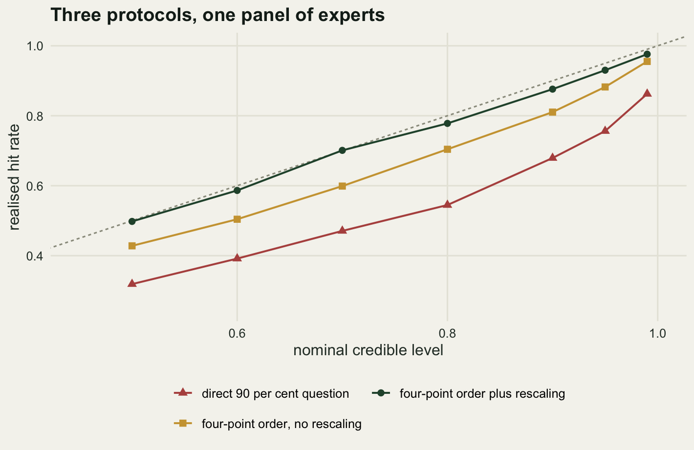
The simulated curves and the analytic ones agree to 0.0425 at worst, so the shape in the figure is the model and not sampling noise. The headline number is the surprise rate. A stated 90 per cent interval from the direct question missed the truth 32.08 per cent of the time, against a nominal 10 per cent. The four-point protocol brings that down to 12.4 per cent, which is better by a factor of about 2.59 and still not right. Overconfidence is the default state of the output, and a protocol that halves it has done well.
The spread across people is what a panel average hides. Under the direct question the worst expert covered 0.4 of the truths and the best covered 0.925; 3 of the 24 had a 90 per cent interval that worked less than half the time.
Here the measurement went against the story. The four-point protocol is not a uniform improvement, because it is a fixed widening applied to people who need different amounts of it. 9 of the 24 experts now cover above nominal rather than below, one of them at 1, and for 2 experts the absolute distance from nominal got worse rather than better. The panel mean deviation still improves, from 0.2229 to 0.0719, so the protocol is worth using. It just converts a panel of overconfident people into a panel split between the two errors, and the ones now above nominal are mostly not the experts who were already fine: 7 of those 9 sat below nominal under the direct question, so the widening over-corrected people who did need correcting.
What the pooling rule actually does
Now the panel has to become one number, or one distribution. Two rules dominate. The linear opinion pool averages the densities:
\[f_L(p) = \sum_{e} w_e f_e(p)\]
and the logarithmic pool multiplies them and renormalises:
\[f_G(p) \propto \prod_{e} f_e(p)^{w_e}\]
These are not two roads to the same place. The linear pool is a mixture, so it keeps every mode any expert had, and by the law of total variance its variance is the average within-expert variance plus the variance of the experts’ centres. Disagreement between experts makes it wider. The logarithmic pool behaves like a product of likelihoods, so for beliefs in the normal family it adds precisions, and disagreement makes it narrower rather than wider, because two people pointing at different places both rule out a great deal.
For beta beliefs about a probability there is a closed form worth knowing. A beta density is proportional to \(p^{a-1}(1-p)^{b-1}\), so the weighted product is proportional to \(p^{\sum w_e (a_e - 1)}(1 - p)^{\sum w_e (b_e - 1)}\), which is another beta with parameters averaged across the panel. That gives an exact answer to check the grid arithmetic against.
Take a panel that has split. Four experts have worked with the population in the drought years and think persistence is unlikely; four have worked with it since and think it is likely. Each holds a beta belief, and the two camps are mirror images.
pg <- seq(1e-4, 1 - 1e-4, length.out = 4001)
dp <- diff(pg)[1]

pool_summ <- function(dens) {
  dens <- dens / (sum(dens) * dp)
  m <- sum(pg * dens) * dp
  cdf <- cumsum(dens) * dp
  c(mean = m, sd = sqrt(sum((pg - m)^2 * dens) * dp),
    lo = pg[which(cdf >= 0.05)[1]], hi = pg[which(cdf >= 0.95)[1]],
    mode = pg[which.max(dens)])
}
n_modes <- function(dens) {
  k <- length(dens)
  mid <- dens[2:(k - 1)]
  sum(mid > dens[1:(k - 2)] & mid > dens[3:k] & mid > 0.02 * max(dens))
}
lin_pool <- function(D, w) as.vector(D %*% w)
log_pool <- function(D, w) {
  g <- exp(as.vector(log(pmax(D, 1e-300)) %*% w))
  g / (sum(g) * dp)
}

a_v <- c(rep(6, 4), rep(18, 4))
b_v <- c(rep(18, 4), rep(6, 4))
w_eq <- rep(1 / length(a_v), length(a_v))
D_split <- sapply(seq_along(a_v), function(i) dbeta(pg, a_v[i], b_v[i]))
L_split <- lin_pool(D_split, w_eq)
G_split <- log_pool(D_split, w_eq)

expert_modes <- (a_v - 1) / (a_v + b_v - 2)
a_bar <- 1 + sum(w_eq * (a_v - 1))
b_bar <- 1 + sum(w_eq * (b_v - 1))

band <- function(s) unname(s[["hi"]] - s[["lo"]])
print(round(rbind(linear = pool_summ(L_split), logarithmic = pool_summ(G_split)), 4))
mean sd lo hi mode
linear 0.5 0.2646 0.1431 0.8569 0.2273
logarithmic 0.5 0.1000 0.3350 0.6650 0.5000print(round(c(linear_width = band(pool_summ(L_split)),
log_width = band(pool_summ(G_split)),
width_ratio = band(pool_summ(L_split)) / band(pool_summ(G_split))), 4))linear_width log_width width_ratio
0.7139 0.3299 2.1636 print(c(modes_linear = n_modes(L_split), modes_log = n_modes(G_split)))modes_linear modes_log
2 1 print(round(c(expert_mode_low = unique(expert_modes)[1],
expert_mode_high = unique(expert_modes)[2],
log_pool_mode = pool_summ(G_split)[["mode"]],
closest_expert_mode_distance =
min(abs(expert_modes - pool_summ(G_split)[["mode"]]))), 4)) expert_mode_low expert_mode_high
0.2273 0.7727
log_pool_mode closest_expert_mode_distance
0.5000 0.2727 print(round(c(closed_form_a = a_bar, closed_form_b = b_bar,
closed_form_mode = (a_bar - 1) / (a_bar + b_bar - 2),
closed_form_sd = sqrt(a_bar * b_bar /
((a_bar + b_bar)^2 * (a_bar + b_bar + 1)))), 4)) closed_form_a closed_form_b closed_form_mode closed_form_sd
12.0 12.0 0.5 0.1 Both pools report a mean of 0.5, because the panel is symmetric and no averaging rule can escape that. Everything else differs. The linear pool gives a 90 per cent band from 0.1431 to 0.8569, a width of 0.7139, with 2 modes: it has reported the disagreement. The logarithmic pool gives 0.335 to 0.665, a width of 0.3299, narrower by a factor of 2.1636, with 1 mode.
That single mode is the thing to look at. It sits at 0.5, and the two camps had modes at 0.2273 and 0.7727. Nobody on this panel thought the most likely value was 0.5; the nearest anyone came was 0.2727 away on the probability scale. The logarithmic pool has manufactured a consensus that is not a summary of anybody’s opinion, and reported it with a 90 per cent band narrower than the linear pool’s. The closed form confirms the arithmetic: the weighted product is Beta(12, 12), whose mode is 0.5 and whose standard deviation is 0.1, matching the grid to four decimal places.
One panel is an anecdote. The sweep below draws 400 random panels of five to nine experts, each belief a beta with a random centre and concentration, and compares the pools on every one.
set.seed(20260731)
n_pan <- 400
sweep_pools <- t(sapply(seq_len(n_pan), function(k) {
  ne <- sample(5:9, 1)
  cen <- rbeta(ne, 2, 2)
  con <- exp(runif(ne, log(6), log(60)))
  D <- sapply(seq_len(ne), function(i) dbeta(pg, cen[i] * con[i],
                                             (1 - cen[i]) * con[i]))
  ww <- rep(1 / ne, ne)
  sL <- pool_summ(lin_pool(D, ww))
  sG <- pool_summ(log_pool(D, ww))
  emod <- (cen * con - 1) / (con - 2)
  c(width_lin = sL[["hi"]] - sL[["lo"]], width_log = sG[["hi"]] - sG[["lo"]],
    sd_lin = sL[["sd"]], sd_log = sG[["sd"]],
    mean_lin = sL[["mean"]], mean_log = sG[["mean"]],
    modes_lin = n_modes(lin_pool(D, ww)), modes_log = n_modes(log_pool(D, ww)),
    log_mode_outside = as.numeric(min(abs(emod - sG[["mode"]])) > 0.05))
}))
sweep_pools <- as.data.frame(sweep_pools)
mean_gap <- abs(sweep_pools$mean_lin - sweep_pools$mean_log)
w_ratio <- sweep_pools$width_lin / sweep_pools$width_log

print(round(c(panels = n_pan,
              fraction_linear_wider = mean(sweep_pools$width_lin >
                                             sweep_pools$width_log),
              fraction_linear_sd_larger = mean(sweep_pools$sd_lin >
                                                 sweep_pools$sd_log),
              median_width_ratio = median(w_ratio),
              min_width_ratio = min(w_ratio),
              max_width_ratio = max(w_ratio)), 4))
panels fraction_linear_wider fraction_linear_sd_larger
400.0000 1.0000 1.0000
median_width_ratio min_width_ratio max_width_ratio
2.2018 1.2212 3.4213 print(round(c(fraction_linear_multimodal = mean(sweep_pools$modes_lin > 1),
fraction_log_multimodal = mean(sweep_pools$modes_log > 1),
fraction_log_mode_no_expert = mean(sweep_pools$log_mode_outside),
mean_absolute_gap_in_pool_mean = mean(mean_gap),
largest_gap_in_pool_mean = max(mean_gap)), 4)) fraction_linear_multimodal fraction_log_multimodal
0.7900 0.0000
fraction_log_mode_no_expert mean_absolute_gap_in_pool_mean
0.3650 0.0381
largest_gap_in_pool_mean
0.1489 ind <- do.call(rbind, lapply(seq_along(a_v), function(i)
data.frame(p = pg, d = D_split[, i], who = paste0("expert", i))))
pools_df <- rbind(
data.frame(p = pg, d = L_split, rule = "linear pool"),
data.frame(p = pg, d = G_split, rule = "logarithmic pool"))
ggplot() +
geom_line(data = ind, aes(p, d, group = who), colour = "#b9b8a8",
linewidth = 0.4) +
geom_line(data = pools_df, aes(p, d, colour = rule, linetype = rule),
linewidth = 0.9) +
scale_colour_manual(values = c(te_pal$forest, te_pal$clay), name = NULL) +
scale_linetype_manual(values = c("solid", "solid"), name = NULL) +
labs(x = "probability that the population persists", y = "density",
title = "Two rules for combining eight experts") +
theme_te()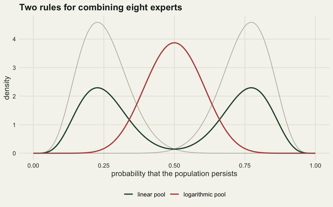
Across all 400 random panels the linear pool was the wider of the two every time, and its standard deviation was the larger every time. The median width ratio was 2.2018 and the ratio ran from 1.2212 to 3.4213. The linear pool was multimodal in 79 per cent of panels and the logarithmic pool in 0 per cent. The split-panel effect is not a special case either: in 36.5 per cent of the random panels the logarithmic mode sat more than 0.05 away on the probability scale from every single expert’s mode.
The centres are not safe either, which is the part that surprises people who assume the pooling rule is a question about spread. The two pools disagreed about the mean by 0.0381 on average and by as much as 0.1489 in the worst panel. On a persistence probability that is the difference between two sentences in a recovery plan.
The rule that falls out of the arithmetic: average the densities if the report should show that the experts disagree, multiply them if you want a working prior for a model that will see data later and you are willing to treat the experts as roughly independent sources of evidence. Choosing the second because it produces a tidier picture is choosing to hide the disagreement.
Performance weights, and what they actually measure
Equal weights are a choice, not the absence of one. Cooke’s classical model replaces them with weights earned on seed questions: quantities with known answers, mixed into the elicitation without being flagged. Each expert’s weight is a product of two scores.
The calibration score asks whether the expert’s quantiles behave like quantiles. With 5, 50 and 95 per cent quantiles the real line splits into four bins, into which the truth should fall with probabilities 0.05, 0.45, 0.45 and 0.05. Compare the observed proportions with those, through twice the number of seeds times the Kullback-Leibler divergence, which is asymptotically chi-square on three degrees of freedom, and take the upper tail probability. Well behaved experts score near one; experts whose truths keep landing outside their 90 per cent range score near zero.
The information score asks how much the expert narrowed things down relative to a uniform background over the intrinsic range of each question. A tight set of quantiles scores high.
The product, with a significance cutoff that zeroes anybody whose calibration score falls below 0.05, is the weight. The decision maker is then the linear pool with those weights, which is what the classical model prescribes.
zqn <- function(q) qnorm(q)

make_panel <- function(seed, n_item, n_exp, world) {
  set.seed(seed)
  s_i <- switch(world,
                skill = exp(rnorm(n_exp, log(0.55), 0.50)),
                exp(rnorm(n_exp, log(0.55), 0.05)))
  ph <- switch(world,
               over = runif(n_exp, 0.30, 1.15),
               runif(n_exp, 0.70, 0.80))
  bi <- rnorm(n_exp, 0, 0.20)
  th <- rnorm(n_item, 0, 1)
  mu <- matrix(th, n_exp, n_item, byrow = TRUE) + bi * s_i +
    matrix(rnorm(n_exp * n_item), n_exp) * s_i
  list(theta = th, mu = mu, sg = ph * s_i, spread = s_i, adjust = ph,
       n_exp = n_exp, n_item = n_item)
}

cooke_scores <- function(pl, idx) {
  th <- pl$theta[idx]
  mu <- pl$mu[, idx, drop = FALSE]
  N <- length(idx)
  q05 <- mu + zqn(0.05) * pl$sg
  q95 <- mu + zqn(0.95) * pl$sg
  thm <- matrix(th, pl$n_exp, N, byrow = TRUE)
  bin <- (thm > q05) + (thm > mu) + (thm > q95) + 1L
  pref <- c(0.05, 0.45, 0.45, 0.05)
  lo_i <- apply(rbind(q05, thm), 2, min)
  hi_i <- apply(rbind(q95, thm), 2, max)
  rng <- hi_i - lo_i
  Lb <- lo_i - 0.1 * rng
  Ub <- hi_i + 0.1 * rng
  span <- matrix(Ub - Lb, 4, N, byrow = TRUE)
  Cs <- numeric(pl$n_exp)
  Is <- numeric(pl$n_exp)
  for (e in seq_len(pl$n_exp)) {
    obs <- tabulate(bin[e, ], 4) / N
    kl <- sum(ifelse(obs > 0, obs * log(obs / pref), 0))
    Cs[e] <- 1 - pchisq(2 * N * kl, df = 3)
    wid <- rbind(q05[e, ] - Lb, mu[e, ] - q05[e, ],
                 q95[e, ] - mu[e, ], Ub - q95[e, ])
    Is[e] <- mean(colSums(pref * log(pref / (wid / span))))
  }
  list(calibration = Cs, information = Is)
}

weights_of <- function(sc, mode, alpha = 0.05) {
  raw <- switch(mode,
                classical = sc$calibration * sc$information *
                  (sc$calibration >= alpha),
                calibration_only = sc$calibration * (sc$calibration >= alpha),
                information_only = sc$information)
  if (sum(raw) <= 0) raw <- rep(1, length(raw))
  raw / sum(raw)
}

log_score <- function(pl, idx, w) {
  thm <- matrix(pl$theta[idx], pl$n_exp, length(idx), byrow = TRUE)
  mean(log(colSums(dnorm(thm, pl$mu[, idx, drop = FALSE], pl$sg) * w)))
}

print(c(lower_quantile_percent = 5, median_percent = 50,
        upper_quantile_percent = 95, chisq_degrees_of_freedom = 3))
lower_quantile_percent median_percent upper_quantile_percent
5 50 95
chisq_degrees_of_freedom
3 print(c(bin_probabilities = c(0.05, 0.45, 0.45, 0.05)))bin_probabilities1 bin_probabilities2 bin_probabilities3 bin_probabilities4
0.05 0.45 0.45 0.05 cor_over <- t(sapply(1:150, function(r) {
pl <- make_panel(41000 + r, 160, 20, "over")
sc <- cooke_scores(pl, 1:20)
c(info_vs_adjust = cor(sc$information, pl$adjust),
calib_vs_adjust = cor(sc$calibration, pl$adjust))
}))
cor_skill <- t(sapply(1:150, function(r) {
pl <- make_panel(52000 + r, 160, 20, "skill")
sc <- cooke_scores(pl, 1:20)
c(info_vs_spread = cor(sc$information, pl$spread),
calib_vs_spread = cor(sc$calibration, pl$spread))
}))
print(round(colMeans(cor_over), 4)) info_vs_adjust calib_vs_adjust
-0.9769 0.5590 print(round(colMeans(cor_skill), 4)) info_vs_spread calib_vs_spread
-0.9531 -0.0162 Before the weights are used for anything, it is worth asking what they correlate with. Two worlds are simulated. In the first, the experts differ only in how much they shrink their intervals: the inner beliefs are equally good, and the variation is pure overconfidence. In the second, the experts differ only in the quality of the inner belief, and everybody reports it with the same shrinkage. Twenty experts, twenty seed questions, 150 repeats of each.
The information score correlates -0.9769 with the shrinkage factor in the first world and -0.9531 with the true belief spread in the second. Those are the same number for two opposite reasons. A narrow set of quantiles earns a high information score whether it is narrow because the expert knows something or narrow because the expert is overconfident, and nothing in the score can separate them. The calibration score can, in principle, which is what the seed questions are for, and it correlates 0.559 with the shrinkage factor. Whether that is enough is a question about sample size.
n_exp_w <- 20
n_item_w <- 160
n_hold <- 50
seed_grid <- c(4, 8, 14, 20, 30, 45, 70, 95)
n_rep <- 60
worlds <- c("skill", "over", "alike")
world_lab <- c(skill = "experts differ in skill",
               over = "experts differ in overconfidence",
               alike = "experts alike")
world_off <- c(skill = 0, over = 3e5, alike = 6e5)

sweep_rows <- list()
for (wd in worlds) {
  for (md in c("classical", "information_only", "calibration_only")) {
    for (ns in seed_grid) {
      adv <- numeric(n_rep)
      eff <- numeric(n_rep)
      for (r in seq_len(n_rep)) {
        pl <- make_panel(1000 * ns + r + world_off[[wd]], n_item_w, n_exp_w, wd)
        set.seed(99000 + r)
        perm <- sample(n_item_w)
        seed_idx <- perm[1:ns]
        hold_idx <- perm[(n_item_w - n_hold + 1):n_item_w]
        w <- weights_of(cooke_scores(pl, seed_idx), md)
        eff[r] <- 1 / sum(w^2)
        adv[r] <- log_score(pl, hold_idx, w) -
          log_score(pl, hold_idx, rep(1 / n_exp_w, n_exp_w))
      }
      sweep_rows[[length(sweep_rows) + 1]] <- data.frame(
        world = wd, scheme = md, n_seed = ns, advantage = mean(adv),
        se = sd(adv) / sqrt(n_rep), win_rate = mean(adv > 0),
        effective_experts = mean(eff))
    }
  }
}
cooke_tab <- do.call(rbind, sweep_rows)
cl <- cooke_tab[cooke_tab$scheme == "classical", ]
show_cols <- c("n_seed", "advantage", "se", "win_rate", "effective_experts")
for (wd in worlds) print(round(cl[cl$world == wd, show_cols], 4))
n_seed advantage se win_rate effective_experts
1 4 0.1374 0.0128 0.9500 12.1588
2 8 0.1428 0.0123 0.9667 11.3297
3 14 0.1230 0.0171 0.8333 9.5847
4 20 0.1067 0.0181 0.8000 8.0981
5 30 0.0965 0.0203 0.7167 6.9208
6 45 0.0375 0.0246 0.6167 5.0450
7 70 -0.0158 0.0302 0.5000 3.3697
8 95 -0.1831 0.0452 0.3500 3.2174
n_seed advantage se win_rate effective_experts
25 4 -0.0099 0.0037 0.3833 12.0028
26 8 -0.0392 0.0049 0.1500 10.1807
27 14 -0.0580 0.0061 0.0833 8.6837
28 20 -0.0705 0.0055 0.0167 7.6131
29 30 -0.0825 0.0072 0.0500 6.1073
30 45 -0.1161 0.0102 0.0167 5.4569
31 70 -0.1035 0.0071 0.0000 4.5052
32 95 -0.1390 0.0090 0.0000 3.7242
n_seed advantage se win_rate effective_experts
49 4 -0.0015 0.0019 0.4500 13.5902
50 8 -0.0002 0.0024 0.6000 13.0429
51 14 -0.0012 0.0024 0.5000 10.8299
52 20 -0.0112 0.0036 0.3500 9.1114
53 30 -0.0156 0.0046 0.3667 7.4460
54 45 -0.0203 0.0048 0.2500 5.4721
55 70 -0.0505 0.0106 0.2500 3.3925
56 95 -0.1435 0.0186 0.0833 2.2649sk <- cl[cl$world == "skill", ]
cross_lo <- max(sk$n_seed[sk$advantage > 0])
cross_hi <- min(sk$n_seed[sk$n_seed > cross_lo])
pick <- function(s, wd) cooke_tab[cooke_tab$scheme == s & cooke_tab$world == wd, ]
io <- pick("information_only", "skill")
co <- pick("calibration_only", "skill")
co_any <- cooke_tab$advantage[cooke_tab$scheme == "calibration_only"]
print(round(c(skill_last_positive_n_seed = cross_lo,
skill_first_negative_n_seed = cross_hi,
info_only_mean_advantage = mean(io$advantage),
info_only_win_rate = mean(io$win_rate),
calib_only_max_advantage = max(co$advantage),
calib_only_best_in_any_world = max(co_any),
calib_only_at_95 = co$advantage[co$n_seed == 95],
effective_experts_at_4 = sk$effective_experts[sk$n_seed == 4],
effective_experts_at_95 = sk$effective_experts[sk$n_seed == 95],
panel_size = n_exp_w), 4)) skill_last_positive_n_seed skill_first_negative_n_seed
45.0000 70.0000
info_only_mean_advantage info_only_win_rate
0.1571 1.0000
calib_only_max_advantage calib_only_best_in_any_world
-0.0047 -0.0032
calib_only_at_95 effective_experts_at_4
-0.2317 12.1588
effective_experts_at_95 panel_size
3.2174 20.0000 cl$world_f <- factor(world_lab[cl$world], levels = unname(world_lab))
ggplot(cl, aes(n_seed, advantage)) +
geom_hline(yintercept = 0, linetype = "22", colour = "#9a9a8c") +
geom_errorbar(aes(ymin = advantage - se, ymax = advantage + se),
width = 0.04, colour = te_pal$sage) +
geom_line(colour = te_pal$forest, linewidth = 0.8) +
geom_point(colour = te_pal$forest, size = 2.1) +
facet_wrap(~world_f, nrow = 1) +
scale_x_log10(breaks = c(4, 10, 30, 95)) +
labs(x = "seed questions used to set the weights",
y = "log score gain over equal weights",
title = "When performance weights pay") +
theme_te() +
theme(legend.position = "none", plot.margin = margin(8, 14, 4, 8))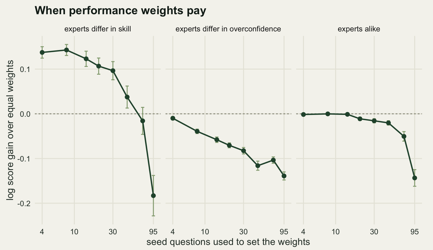
The left panel is the case the classical model was built for, and it delivers: with 4 seed questions the weighted decision maker beats the equal-weight one by 0.1374 in mean held-out log density, winning in 95 per cent of repeats. In the middle panel, where the only difference between experts is how overconfident they are, the weights lose at every seed count tested, from -0.0099 at 4 seeds to -0.139 at 95. The right panel, where the experts are interchangeable, starts at break-even and gets worse.
Then the result that goes the wrong way. The advantage in the skill world does not grow with the number of seed questions; it shrinks, crosses zero between 45 and 70 seeds, and is -0.1831 by 95 seeds. More evidence about who is good makes the weighting worse.
The decomposition says why. The information score, which never looks at a truth and therefore does not care how many seed questions there are, is doing all of the winning: on its own it gains between 0.1492 and 0.1645 in the skill world at every seed count, winning 100 per cent of the time. The calibration score, the only part that uses the answers, never has a positive mean advantage in that world at all: its best is -0.0047 and it reaches -0.2317 at 95 seeds. What the calibration factor does as the seeds accumulate is concentrate the panel. The effective number of experts, one over the sum of squared weights, falls from 12.1588 at 4 seeds to 3.2174 at 95, out of 20. A pool that rests on two or three people has the variance of two or three people.
So the threshold exists but runs backwards from the way it is usually described. It is not a minimum number of seed questions below which the weights are too noisy to trust; it is a maximum, past which the calibration score becomes decisive enough to collapse the panel onto a handful of survivors. Cooke’s own practice of optimising the cutoff on the seed set answers the same problem from the other direction, and the version above, with the cutoff fixed at 0.05, is the version most people implement.
One caveat belongs here rather than at the end. The held-out score used above is the log density of a mixture, and a mixture is rewarded for having one sharp component near the truth. That is a real property of the linear pool, but it does mean the information score is being judged on the thing it optimises; change the target to one that punishes sharpness and the ranking would move.
Does any of this reach the decision
A number that changes nothing is not worth arguing about. The elicited quantity here is the mean annual growth rate on the log scale of a reintroduced population, and the decision is between translocating founders to a new site and spending the same money protecting the remnant where it is. Translocation succeeds if the founded population exceeds a threshold after twenty years, which under a simple diffusion happens with probability
\[V_A(r) = \Phi\!\left(\frac{\log n_0 + T r - \log N_{\text{crit}}} {\sigma_{\text{env}}\sqrt{T}}\right)\]
and protecting in place has a known value \(v_B\), because that population has been monitored for decades. Here the width of the elicited distribution matters on its own, separately from where it is centred, because \(V_A\) is not linear in \(r\). For a normal belief about \(r\) the expectation is available in closed form: the environmental variance and the belief variance add under the normal integral, so a narrower belief means a smaller denominator, which pushes \(\Phi\) further towards zero or one depending on the sign of the numerator.
That sign is the whole story. \(\Phi\) has its inflection where the argument is zero, which is where the panel thinks translocation is an even bet. Below that point the value function is convex and overconfidence makes the option look worse; above it the function is concave and overconfidence makes it look better. Bias moves the centre instead, and moving the centre moves the answer wherever you are.
set.seed(20260806)
n_panel <- 8000
n_expert <- 12
n0 <- 30
t_yr <- 20
n_crit <- 50
sig_env <- 0.18

ev_translocate <- function(mu, sd) {
  mean(pnorm((log(n0) + t_yr * mu - log(n_crit)) /
               sqrt(t_yr * sig_env^2 + t_yr^2 * sd^2)))
}

panels <- lapply(seq_len(n_panel), function(k) {
  r_true <- rnorm(1, 0.025, 0.035)
  s_i <- exp(rnorm(n_expert, log(0.030), 0.35))
  ph <- runif(n_expert, 0.35, 0.85)
  bi <- rnorm(n_expert, 0, 0.45)
  eps <- rnorm(n_expert) * s_i
  list(mu_clean = r_true + eps, mu_biased = r_true + bi * s_i + eps,
       sd_true = s_i, sd_narrow = ph * s_i)
})

ev <- as.data.frame(t(sapply(panels, function(p) c(
  calibrated = ev_translocate(p$mu_clean, p$sd_true),
  overconfident = ev_translocate(p$mu_clean, p$sd_narrow),
  biased = ev_translocate(p$mu_biased, p$sd_true),
  both = ev_translocate(p$mu_biased, p$sd_narrow)))))

print(round(c(panels = n_panel, experts_per_panel = n_expert,
              founders = n0, horizon_years = t_yr, threshold = n_crit,
              environmental_sd = sig_env), 4))
panels experts_per_panel founders horizon_years
8000.00 12.00 30.00 20.00
threshold environmental_sd
50.00 0.18 print(round(c(mean_calibrated_value = mean(ev$calibrated),
sd_across_panels = sd(ev$calibrated),
shift_overconfident = mean(abs(ev$overconfident - ev$calibrated)),
shift_biased = mean(abs(ev$biased - ev$calibrated)),
shift_both = mean(abs(ev$both - ev$calibrated)),
fraction_overconfidence_raised_value =
mean(ev$overconfident > ev$calibrated)), 4)) mean_calibrated_value sd_across_panels
0.4995 0.2119
shift_overconfident shift_biased
0.0137 0.0191
shift_both fraction_overconfidence_raised_value
0.0226 0.5018 Overconfidence moves the expected value of translocation by 0.0137 on average, bias by 0.0191, and the two together by 0.0226. Overconfidence pushed the value up in 50.18 per cent of panels and down in the rest, which is the two-sided behaviour the inflection point predicts and the reason it never shows up as a bias in an average across projects.
Whether a shift of that size changes anything depends on how close the decision was. Sweeping the value of the in-place option across the range a real programme might occupy, and recording how often the flawed elicitation picks the other option, gives the rate directly. The second sweep restricts to close calls: panels where the calibrated expected value lands within 0.05 of the in-place option, which is where a decision analyst would already be nervous.
v_grid <- seq(0.25, 0.80, by = 0.025)
flip <- function(nm, v, keep) {
  mean((ev$calibrated[keep] > v) != (ev[[nm]][keep] > v))
}
switch_tab <- do.call(rbind, lapply(v_grid, function(v) {
  near <- abs(ev$calibrated - v) < 0.05
  data.frame(v_place = v, n_close = sum(near),
             overconfident_all = flip("overconfident", v, rep(TRUE, n_panel)),
             biased_all = flip("biased", v, rep(TRUE, n_panel)),
             overconfident_close = flip("overconfident", v, near),
             biased_close = flip("biased", v, near),
             both_close = flip("both", v, near))
}))
print(round(switch_tab[seq(1, nrow(switch_tab), by = 3), ], 4))
v_place n_close overconfident_all biased_all overconfident_close
1 0.250 890 0.0229 0.0238 0.2056
4 0.325 1053 0.0171 0.0254 0.1301
7 0.400 1213 0.0156 0.0306 0.1031
10 0.475 1310 0.0058 0.0349 0.0351
13 0.550 1248 0.0066 0.0332 0.0425
16 0.625 1180 0.0179 0.0285 0.1212
19 0.700 1047 0.0235 0.0270 0.1796
22 0.775 811 0.0226 0.0192 0.2232
biased_close both_close
1 0.2101 0.2258
4 0.1871 0.2118
7 0.1937 0.2168
10 0.2053 0.2107
13 0.2115 0.2099
16 0.1881 0.2220
19 0.2044 0.2311
22 0.1887 0.2256oc <- switch_tab$overconfident_close
bc <- switch_tab$biased_close
v_min <- switch_tab$v_place[which.min(oc)]
print(round(c(overconfident_close_mean = mean(oc),
overconfident_close_min = min(oc),
overconfident_close_min_at = v_min,
overconfident_close_max = max(oc),
overconfident_close_max_at = switch_tab$v_place[which.max(oc)]), 4)) overconfident_close_mean overconfident_close_min
0.1200 0.0261
overconfident_close_min_at overconfident_close_max
0.5250 0.2252
overconfident_close_max_at
0.8000 print(round(c(biased_close_mean = mean(bc), biased_close_min = min(bc),
biased_close_max = max(bc),
biased_close_range = max(bc) - min(bc),
overconfident_close_range = max(oc) - min(oc)), 4)) biased_close_mean biased_close_min biased_close_max
0.1962 0.1642 0.2266
biased_close_range overconfident_close_range
0.0625 0.1991 print(round(c(both_close_mean = mean(switch_tab$both_close),
overconfident_all_mean = mean(switch_tab$overconfident_all),
biased_all_mean = mean(switch_tab$biased_all)), 4)) both_close_mean overconfident_all_mean biased_all_mean
0.2174 0.0154 0.0279 lab_d <- c("overconfidence only", "bias only")
sw_long <- rbind(
data.frame(v_place = switch_tab$v_place, rate = oc, flaw = lab_d[1]),
data.frame(v_place = switch_tab$v_place, rate = bc, flaw = lab_d[2]))
sw_long$flaw <- factor(sw_long$flaw, levels = lab_d)
ggplot(sw_long, aes(v_place, rate, colour = flaw, shape = flaw)) +
geom_line(linewidth = 0.8) +
geom_point(size = 2.1) +
scale_colour_manual(values = c(te_pal$forest, te_pal$clay), name = NULL) +
scale_shape_manual(values = c(16, 17), name = NULL) +
labs(x = "value of protecting the remnant in place",
y = "fraction of close calls that flip",
title = "Which flaw changes the decision") +
theme_te() +
theme(plot.margin = margin(8, 14, 4, 8))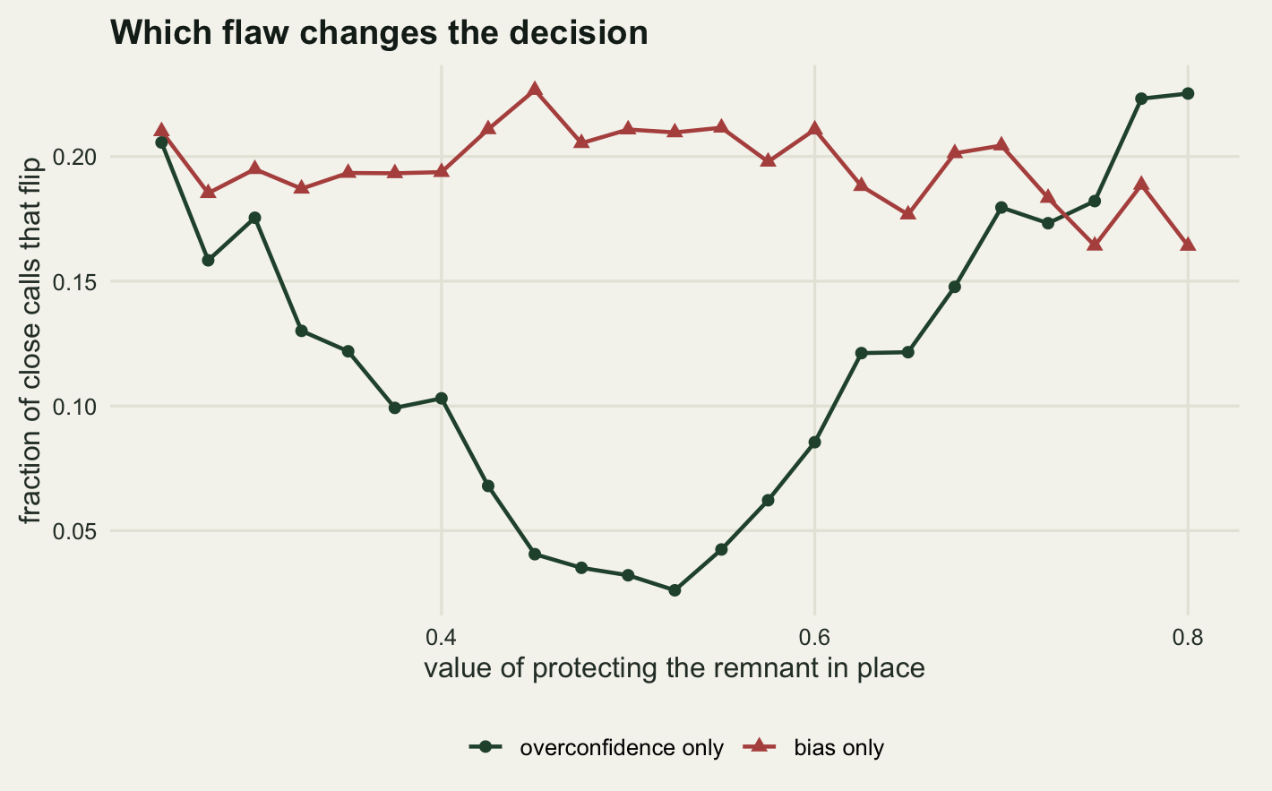
Among close calls, overconfidence alone flipped the choice in 12 per cent of panels on average across the sweep, but the average is the least interesting number in the figure. The rate falls to 2.61 per cent when the in-place option is worth 0.525, near where the panel’s own expected value of translocation sits, and rises to 22.52 per cent at the right-hand end. The range across the sweep is 19.91 percentage points.
Bias behaves completely differently. It flips 19.62 per cent of close calls on average with a range of only 6.25 percentage points across the same sweep: a flat line where overconfidence is a U. Averaged over the sweep bias is the larger problem, 19.62 per cent against 12 per cent, and the two together flip 21.74 per cent.
The practical version: if the panel is genuinely torn about the option in front of them their overconfidence will not change what you decide and their standing bias will, while if the panel leans one way and the alternative is close in value anyway, overconfidence is what pushes you over the line, in whichever direction the panel already leaned. Widening everyone’s intervals by protocol does nothing for the first case and helps in the second.
What to take away
An elicited probability is an output of a procedure, and the procedure has measurable properties. Asking for bounds before the best guess lifted realised coverage by 0.1312 and adding the confidence question lifted it by a further 0.0656, leaving a surprise rate of 12.4 per cent against a nominal 10 per cent. Overconfidence is not eliminated by any of this; it is reduced by about a factor of 2.59.
Three of the measurements went against the direction I expected. The four-point protocol made 2 of 24 experts worse rather than better, because it applies a fixed widening to people who need different amounts of it, and it turned 7 of them from overconfident into underconfident. Performance weights did best with the fewest seed questions and crossed into losing between 45 and 70 of them, because the part of the weight that uses the answers concentrates the panel from 12.1588 effective experts down to 3.2174 without buying accuracy. And bias, not overconfidence, was the flaw that changed the most decisions: 19.62 per cent of close calls against 12 per cent, even though overconfidence is the failure the protocols are all built to fight.
The pooling result is the one to carry into a meeting. A logarithmic pool of a split panel put its mode at 0.5 when the two camps sat at 0.2273 and 0.7727, and reported a 90 per cent band 2.1636 times narrower than the linear pool of the same people. Across 400 random panels the logarithmic mode sat away from every expert’s mode 36.5 per cent of the time. If the pooled number is going into a document that says the experts agreed, the pooling rule needs to be in the document too.
The honest limit is the one this whole post is built on. Every measurement above knows the truth and knows each expert’s real internal belief, and separates protocol damage from ignorance by comparing the two. In a real elicitation neither is available: the quantity is unknown, which is why you asked, and the inner belief is unobservable in principle. Seed questions are the only bridge, and the fourth section measured what it is worth: the best mean advantage the calibration factor reached in any of the three worlds was -0.0032, and the part that carried the gains, the information score, correlated -0.9769 with the interval-shrinkage factor and -0.9531 with the true belief spread, which means it cannot tell them apart. Nothing in this post identifies a real overconfident expert. It identifies what happens downstream if one is in the room.
References
Cooke RM 1991 Experts in Uncertainty: Opinion and Subjective Probability in Science (ISBN 978-0-19-506465-0)
Clemen RT, Winkler RL 1999 Risk Analysis 19(2):187-203 (10.1111/j.1539-6924.1999.tb00399.x)
Speirs-Bridge A, Fidler F, McBride M, Flander L, Cumming G, Burgman M 2010 Risk Analysis 30(3):512-523 (10.1111/j.1539-6924.2009.01337.x)
Martin TG, Burgman MA, Fidler F, Kuhnert PM, Low-Choy S, McBride M, Mengersen K 2012 Conservation Biology 26(1):29-38 (10.1111/j.1523-1739.2011.01806.x)
McBride MF, Garnett ST, Szabo JK, Burbidge AH, Butchart SHM, Christidis L, Dutson G, Ford HA, Loyn RH, Watson DM, Burgman MA 2012 Methods in Ecology and Evolution 3(5):906-920 (10.1111/j.2041-210X.2012.00221.x)
Morgan MG 2014 Proceedings of the National Academy of Sciences 111(20):7176-7184 (10.1073/pnas.1319946111)
Colson AR, Cooke RM 2017 Reliability Engineering and System Safety 163:109-120 (10.1016/j.ress.2017.02.003)
Hemming V, Burgman MA, Hanea AM, McBride MF, Wintle BC 2018 Methods in Ecology and Evolution 9(1):169-180 (10.1111/2041-210X.12857)
O’Hagan A 2019 The American Statistician 73(sup1):69-81 (10.1080/00031305.2018.1518265)