Calibrating predicted probabilities in R

Reliability diagrams, the Brier decomposition, Platt scaling and isotonic regression in base R for occupancy models whose probabilities cannot be trusted.

A distribution model that puts a plot at 0.3 is making a claim you can go and check. Collect every plot the model scored near 0.3, survey them, and about three in ten should hold the species. If seven in ten do, the map may still rank plots correctly and may still be worth having, but the number printed on it is not a probability. Everything built on top of it is then wrong by an amount nobody has measured: the expected number of occupied patches in a region, the threshold above which a site gets surveyed, the cost calculation that decides a management budget.

The trouble is that the summary most of us report cannot see any of this. AUC is a statement about ordering, and ordering survives any monotone squeeze or stretch of the predicted probabilities. Two models with the same AUC can disagree by a factor of five about how many plots to survey. This tutorial measures that, and then repairs it.

Two related tutorials already exist on this blog and are not repeated here. The scoring rules themselves, what the Brier score is and how it relates to the CRPS, are in The CRPS and the Brier score; the calibration of prediction intervals, meaning coverage and PIT histograms, is in Checking predictive calibration. This post is about a single binary probability: how to measure whether it means what it says, and what to do when it does not. The Brier score appears here only in its decomposed form, as the mean of (p - y)^2 split into parts.

Four things get measured below. How much of a reliability diagram is an artefact of the binning you chose. How the Brier score splits exactly into reliability, resolution and uncertainty. What three characteristic kinds of miscalibration do to the Brier score while leaving AUC untouched to the last decimal. And what it costs, in held-out plots, to fit a repair with Platt scaling or with isotonic regression.

library(ggplot2)

te_pal <- list(forest = "#275139", green = "#2f8f63", sage = "#93a87f",
               clay = "#b5534e", gold = "#cda23f", line = "#dad9ca",
               ink = "#16241d", paper = "#f5f4ee")

theme_te <- function() {
  theme_minimal(base_size = 12) +
    theme(panel.grid.minor = element_blank(),
          panel.grid.major = element_line(colour = "#e7e6dc"),
          plot.background = element_rect(fill = "#f5f4ee", colour = NA),
          panel.background = element_rect(fill = "#f5f4ee", colour = NA),
          plot.title = element_text(face = "bold", colour = te_pal$ink),
          axis.title = element_text(colour = "#2c3a31"))
}

Three sets of plots, and a binning by hand

The simulated survey is a saproxylic beetle in forest plots. Occupancy depends on deadwood volume and canopy openness through a logistic model, so the true probability of each plot is known and the model is correctly specified. Three sets of plots are drawn: a training set to fit the model, a calibration set on which every repair below is fitted, and a large test set on which every number below is measured. Nothing is ever measured on the data it was fitted to, for a reason that gets its own section at the end.

set.seed(20260815)
n_train <- 6000; n_cal <- 4000; n_test <- 40000

sim_plots <- function(nn) {
  deadwood <- rnorm(nn)
  openness <- rnorm(nn)
  pt <- plogis(-1.0 + 1.3 * deadwood + 0.7 * openness)
  data.frame(deadwood = deadwood, openness = openness,
             p_true = pt, y = rbinom(nn, 1, pt))
}
train  <- sim_plots(n_train)
calset <- sim_plots(n_cal)
test   <- sim_plots(n_test)

fit <- glm(y ~ deadwood + openness, data = train, family = binomial)
calset$p_fit <- predict(fit, newdata = calset, type = "response")
test$p_fit   <- predict(fit, newdata = test,   type = "response")

cat(sprintf("plots: training %d, calibration %d, test %d\n", n_train, n_cal, n_test))

plots: training 6000, calibration 4000, test 40000

cat(sprintf("occupancy rate: training %.4f, test %.4f\n", mean(train$y), mean(test$y)))

occupancy rate: training 0.3285, test 0.3254

cat(sprintf("fitted logit coefficients: %s\n",
            paste(sprintf("%.3f", coef(fit)), collapse = "  ")))

fitted logit coefficients: -0.989  1.274  0.672

cat(sprintf("largest gap between fitted and true probability on test: %.4f\n",
            max(abs(test$p_fit - test$p_true))))

largest gap between fitted and true probability on test: 0.0160

A reliability diagram needs bins. Sort the plots by predicted probability, cut them into groups of equal size, and in each group compare the mean prediction with the observed occupancy. Ties are kept in the same bin, which matters later because isotonic regression produces heavily tied predictions. The summary usually attached to the diagram is the mean absolute gap between the two, weighted by bin size.

bin_index <- function(pv, nb) {
  rk <- rank(pv, ties.method = "min")
  pmin(pmax(as.integer(ceiling(rk / length(pv) * nb)), 1L), nb)
}
bin_stats <- function(bi, pv, yv, nb) {
  nk <- tabulate(bi, nbins = nb)
  ub <- sort(unique(bi))
  sp <- numeric(nb); sy <- numeric(nb)
  sp[ub] <- as.vector(rowsum(pv, bi, reorder = TRUE))
  sy[ub] <- as.vector(rowsum(yv, bi, reorder = TRUE))
  keep <- nk > 0
  data.frame(nk = nk[keep], pbar = sp[keep] / nk[keep], obar = sy[keep] / nk[keep])
}
cal_error <- function(bi, pv, yv, nb) {
  b <- bin_stats(bi, pv, yv, nb)
  sum(b$nk * abs(b$pbar - b$obar)) / length(yv)
}

The bin count is a knob, and it turns the answer

Take the true probabilities themselves as the predictions. These are calibrated by construction, exactly and by definition, because the outcomes were drawn from them. Any calibration error they show is sampling noise. Compute the error under 5, 10 and 20 bins, and beside it the same quantity under 400 replicate draws of the outcomes from those same probabilities, which is the correct null: how far a perfectly calibrated model wanders by chance at this sample size.

set.seed(20260901)
p_perfect <- test$p_true
nb_set <- c(5, 10, 20)
n_null <- 400
ece_tab <- data.frame()
for (nb in nb_set) {
  bi <- bin_index(p_perfect, nb)
  obs <- cal_error(bi, p_perfect, test$y, nb)
  nulls <- replicate(n_null, cal_error(bi, p_perfect,
                                       rbinom(n_test, 1, p_perfect), nb))
  ece_tab <- rbind(ece_tab, data.frame(
    bins = nb, ece = obs, null_median = median(nulls),
    null_95 = unname(quantile(nulls, 0.95)),
    pctile = mean(nulls <= obs)))
}
cat(sprintf("null replicates per bin count: %d\n", n_null))

null replicates per bin count: 400

print(format(ece_tab, digits = 4), row.names = FALSE)

 bins      ece null_median  null_95 pctile
    5 0.004192    0.003422 0.005601  0.760
   10 0.005686    0.004738 0.006870  0.775
   20 0.008223    0.006788 0.009139  0.845

cat(sprintf("ECE ratio, 20 bins over 5 bins: %.2f\n",
            ece_tab$ece[3] / ece_tab$ece[1]))

ECE ratio, 20 bins over 5 bins: 1.96

The same predictions, on the same 40000 plots, score 0.004192 at 5 bins and 0.008223 at 20 bins: a ratio of 1.96 for a model that is perfect either way. The metric rewards coarse bins, because a coarse bin averages away the very departures the diagram exists to show. A calibration error quoted without its bin count is not a measurement.

The null column is what rescues the situation. At every bin count the observed value sits close to the median of the null and inside its upper 5 percent point (0.005601, 0.006870 and 0.009139), landing at the 0.760, 0.775 and 0.845 percentiles of their own null distributions. Simulating the calibrated case costs a few lines and turns an uninterpretable number into a test.

set.seed(20260902)
band_rows <- list()
for (nb in nb_set) {
  bi <- bin_index(p_perfect, nb)
  b <- bin_stats(bi, p_perfect, test$y, nb)
  sims <- replicate(n_null, bin_stats(bi, p_perfect,
                                      rbinom(n_test, 1, p_perfect), nb)$obar)
  band_rows[[length(band_rows) + 1]] <- data.frame(
    panel = sprintf("%d bins (error %.4f)", nb, ece_tab$ece[ece_tab$bins == nb]),
    pbar = b$pbar, obar = b$obar,
    lo = apply(sims, 1, quantile, 0.025),
    hi = apply(sims, 1, quantile, 0.975))
}
rel_dat <- do.call(rbind, band_rows)
rel_dat$panel <- factor(rel_dat$panel, levels = unique(rel_dat$panel))
cat(sprintf("widest 95 percent null interval, 20 bins: %.4f\n",
            max(rel_dat$hi[grepl("^20", rel_dat$panel)] -
                  rel_dat$lo[grepl("^20", rel_dat$panel)])))

widest 95 percent null interval, 20 bins: 0.0440

ggplot(rel_dat, aes(pbar, obar - pbar)) +
  geom_hline(yintercept = 0, linetype = "dashed", colour = te_pal$ink) +
  geom_ribbon(aes(ymin = lo - pbar, ymax = hi - pbar), fill = te_pal$sage,
              alpha = 0.55) +
  geom_line(colour = te_pal$forest, linewidth = 0.8) +
  geom_point(colour = te_pal$forest, size = 1.8) +
  facet_wrap(~ panel) +
  labs(title = "A perfectly calibrated model, binned three ways",
       x = "mean predicted probability in bin",
       y = "observed occupancy minus prediction") +
  theme_te()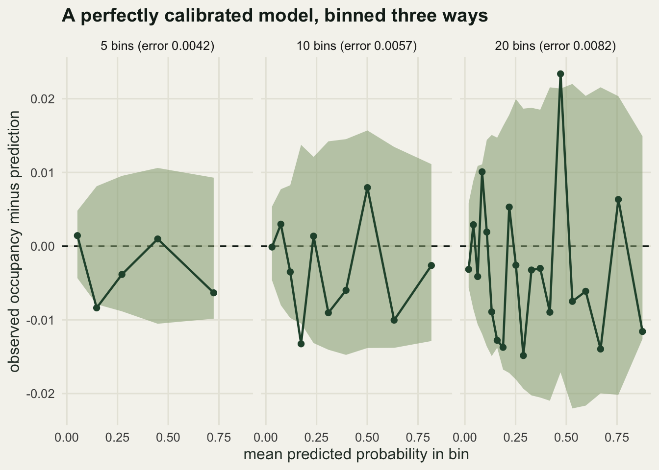

Departure from the diagonal for a perfectly calibrated predictor under three bin counts, with a 95 percent null band from 400 replicate outcome draws. Plotting the gap rather than the raw diagram is the only way to see a band this narrow.

The widest null interval in the 20 bin panel spans 0.0440 of occupancy. That is the amount of apparent miscalibration you should expect to see, in the worst bin, from a model that has nothing wrong with it, on forty thousand plots. On the two hundred plots of a real survey the band would swallow the diagram whole.

Splitting the Brier score into three pieces

Murphy’s decomposition writes the Brier score of a binned forecast as reliability minus resolution plus uncertainty. Reliability is the size-weighted squared gap between the mean prediction and the observed frequency in each bin, and smaller is better. Resolution is the size-weighted squared distance of each bin’s observed frequency from the overall occupancy rate, and larger is better: it is the model’s ability to separate plots at all. Uncertainty is the occupancy rate times one minus itself, a property of the landscape that no model can change.

The identity is exact when the forecast being scored is the bin mean, so the code below scores both: the raw continuous predictions, and the same predictions rounded to their bin means. The residual of the identity is printed as the check.

murphy <- function(pv, yv, nb) {
  bidx <- bin_index(pv, nb)
  bs <- bin_stats(bidx, pv, yv, nb)
  nn <- length(yv); obar <- mean(yv)
  reli <- sum(bs$nk * (bs$pbar - bs$obar)^2) / nn
  reso <- sum(bs$nk * (bs$obar - obar)^2) / nn
  unce <- obar * (1 - obar)
  bs_bin <- mean((bs$pbar[bidx] - yv)^2)
  c(reliability = reli, resolution = reso, uncertainty = unce,
    brier_binned = bs_bin, brier_raw = mean((pv - yv)^2),
    residual = bs_bin - (reli - reso + unce))
}
mur_tab <- as.data.frame(t(sapply(nb_set, function(nb) murphy(test$p_fit, test$y, nb))))
mur_tab$bins <- nb_set
mur_tab <- mur_tab[, c("bins", "reliability", "resolution", "uncertainty",
                       "brier_binned", "brier_raw", "residual")]
print(format(mur_tab, digits = 5), row.names = FALSE)

 bins reliability resolution uncertainty brier_binned brier_raw    residual
    5  3.2421e-05   0.056110     0.21951      0.16344   0.15968 -1.1102e-16
   10  4.6605e-05   0.058990     0.21951      0.16057   0.15968  2.7756e-17
   20  9.1979e-05   0.059686     0.21951      0.15992   0.15968  8.3267e-17

cat(sprintf("largest absolute residual of the identity: %.3e\n",
            max(abs(mur_tab$residual))))

largest absolute residual of the identity: 1.110e-16

cat(sprintf("binning cost at 5 bins: %.5f; at 20 bins: %.5f\n",
            mur_tab$brier_binned[1] - mur_tab$brier_raw[1],
            mur_tab$brier_binned[3] - mur_tab$brier_raw[3]))

binning cost at 5 bins: 0.00375; at 20 bins: 0.00024

At 10 bins the fitted model has reliability 4.6605e-05, resolution 0.058990 and uncertainty 0.21951, giving a binned Brier score of 0.16057, and the residual of the identity is -2.7756e-17. That is machine precision, which is the point of printing it: an implementation of a decomposition that does not close to machine precision has a bug in it, and this is the cheapest available way to find out.

The last line is the same coarse-bin problem seen from the other side. Rounding predictions to their bin means costs 0.00375 of Brier score at 5 bins and only 0.00024 at 20. Coarse bins flatter the calibration error precisely because they throw resolution away, and the Brier score, which counts both, notices.

Three shapes of wrong, one AUC

Now break the predictions on purpose, in the three ways models actually break. Each distortion is applied in logit space to the same fitted scores.

Overconfidence multiplies the logit by 1.9, pushing predictions towards 0 and 1. This is what a model does when it has been fitted with too little regularisation or on too few plots, and it is the failure mode of a boosted ensemble. Underconfidence shrinks the logit towards the base rate by a factor of 0.45, the characteristic shape of a bagged ensemble that averages votes: an average of many noisy votes cannot get near 0 or 1. Bias adds 0.9 to every logit, which is roughly what happens when a model is fitted on a downsampled dataset with the absences thinned and the correction is never applied.

A fourth is added because it is needed in the next section: a wavy distortion that adds 0.8 * sin(logit), still monotone but not a straight line in logit space. It stands for a model that is calibrated in the middle of its range and drifts at both ends.

lg <- function(x) log(x / (1 - x))
base_rate <- mean(train$y)
warp <- list(
  calibrated     = function(q) q,
  overconfident  = function(q) plogis(1.9 * lg(q)),
  underconfident = function(q) plogis(lg(base_rate) + 0.45 * (lg(q) - lg(base_rate))),
  biased         = function(q) plogis(lg(q) + 0.9),
  wavy           = function(q) plogis(lg(q) + 0.8 * sin(lg(q))))

auc_rank <- function(pv, yv) {
  rk <- rank(pv)
  n1 <- as.numeric(sum(yv == 1)); n0 <- as.numeric(sum(yv == 0))
  (sum(rk[yv == 1]) - n1 * (n1 + 1) / 2) / (n1 * n0)
}
rel_comp <- function(pv, yv, nb = 10) {
  b <- bin_stats(bin_index(pv, nb), pv, yv, nb)
  sum(b$nk * (b$pbar - b$obar)^2) / length(yv)
}

shp_tab <- do.call(rbind, lapply(names(warp), function(nm) {
  qq <- warp[[nm]](test$p_fit)
  data.frame(shape = nm, brier = mean((qq - test$y)^2),
             reliability = rel_comp(qq, test$y), auc = auc_rank(qq, test$y),
             mean_prediction = mean(qq))
}))
print(format(shp_tab, digits = 6), row.names = FALSE)

          shape    brier reliability      auc mean_prediction
     calibrated 0.159684 4.66048e-05 0.812198        0.328679
  overconfident 0.168891 8.96226e-03 0.812198        0.282315
 underconfident 0.173408 1.36188e-02 0.812198        0.317364
         biased 0.188529 2.87815e-02 0.812198        0.484616
           wavy 0.164768 4.89139e-03 0.812198        0.299138

cat(sprintf("spread of AUC across the five predictors: %.3e\n",
            diff(range(shp_tab$auc))))

spread of AUC across the five predictors: 0.000e+00

cat(sprintf("test-set occupancy rate for comparison: %.4f\n", mean(test$y)))

test-set occupancy rate for comparison: 0.3254

The Brier score moves a long way: 0.159684 for the calibrated predictor, 0.168891 overconfident, 0.173408 underconfident, 0.188529 biased. The reliability component moves further in relative terms, from 4.66048e-05 to 0.0287815, a factor of over six hundred. The mean prediction, which is what you would sum to get an expected number of occupied plots, runs from 0.282315 to 0.484616 against a true occupancy rate of 0.3254.

And the AUC is 0.812198 for all five. Not approximately: the spread across the five is 0.000e+00. Every distortion here is a strictly increasing function of the original score, so the ranking is untouched, and AUC is a functional of the ranking alone. The single number most often reported for a distribution model is blind, by construction, to every failure in this table.

nb_show <- 20
shape_lv <- names(warp)
curve_dat <- do.call(rbind, lapply(shape_lv, function(nm) {
  qq <- warp[[nm]](test$p_fit)
  b <- bin_stats(bin_index(qq, nb_show), qq, test$y, nb_show)
  data.frame(shape = factor(nm, levels = shape_lv), pbar = b$pbar, obar = b$obar)
}))
ggplot(curve_dat, aes(pbar, obar, colour = shape)) +
  geom_abline(slope = 1, intercept = 0, linetype = "dashed", colour = te_pal$ink) +
  geom_line(linewidth = 0.9) + geom_point(size = 1.6) +
  scale_colour_manual(values = c(te_pal$ink, te_pal$clay, te_pal$gold,
                                 te_pal$green, te_pal$forest)) +
  coord_cartesian(xlim = c(0, 1), ylim = c(0, 1)) +
  labs(title = "Five predictors, one AUC",
       x = "mean predicted probability in bin",
       y = "observed occupancy in bin", colour = NULL) +
  theme_te() + theme(legend.position = "top")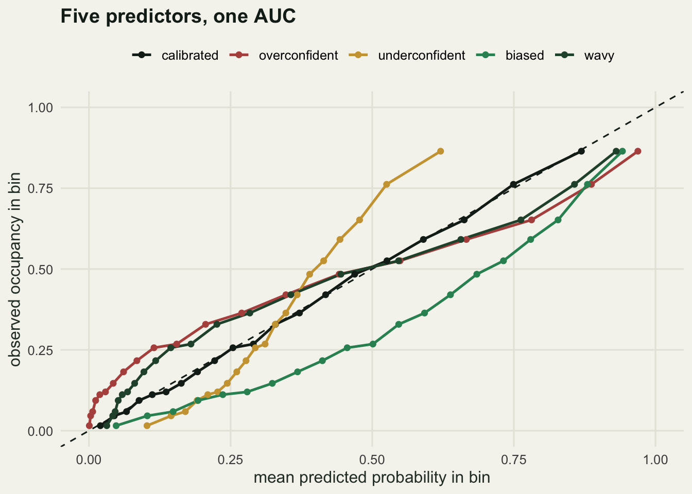

Reliability curves at 20 bins for five predictors that share an identical AUC of 0.812198. Only the calibrated one follows the diagonal.

Two repairs, written out

Platt scaling is a logistic regression of the outcome on the logit of the predicted probability, fitted on held-out data. Two parameters, an intercept and a slope; the fitted map is a straight line in logit space. It is written here as iteratively reweighted least squares so that nothing is hidden, and checked against glm.

Isotonic regression asks only for a monotone map and finds the best one by least squares. The algorithm is pool adjacent violators: walk up the sorted predictions carrying a stack of blocks, and whenever the new block is lower than the one below it, merge them into their weighted mean and check again. The result is a step function of the score.

platt_fit <- function(pv, yv) {
  eps <- 1e-6
  xmat <- cbind(1, lg(pmin(pmax(pv, eps), 1 - eps)))
  bcoef <- c(0, 0)
  for (it in 1:50) {
    eta <- as.vector(xmat %*% bcoef)
    mu <- plogis(eta)
    wv <- pmax(mu * (1 - mu), 1e-10)
    zwork <- eta + (yv - mu) / wv
    bnew <- as.vector(solve(crossprod(xmat * wv, xmat), crossprod(xmat * wv, zwork)))
    if (max(abs(bnew - bcoef)) < 1e-10) { bcoef <- bnew; break }
    bcoef <- bnew
  }
  bcoef
}
platt_apply <- function(bcoef, pv) {
  eps <- 1e-6
  plogis(bcoef[1] + bcoef[2] * lg(pmin(pmax(pv, eps), 1 - eps)))
}

pava <- function(yv, wv) {
  nn <- length(yv)
  lev <- numeric(nn); wgt <- numeric(nn); cnt <- integer(nn); kk <- 0L
  for (i in seq_len(nn)) {
    kk <- kk + 1L
    lev[kk] <- yv[i]; wgt[kk] <- wv[i]; cnt[kk] <- 1L
    while (kk > 1L && lev[kk - 1L] > lev[kk]) {
      wsum <- wgt[kk - 1L] + wgt[kk]
      lev[kk - 1L] <- (wgt[kk - 1L] * lev[kk - 1L] + wgt[kk] * lev[kk]) / wsum
      wgt[kk - 1L] <- wsum
      cnt[kk - 1L] <- cnt[kk - 1L] + cnt[kk]
      kk <- kk - 1L
    }
  }
  rep(lev[seq_len(kk)], cnt[seq_len(kk)])
}
iso_fit <- function(pv, yv) {
  o <- order(pv)
  ps <- pv[o]
  gs <- pava(yv[o], rep(1, length(yv)))
  last <- !duplicated(ps, fromLast = TRUE)
  list(x = ps[last], g = gs[last])
}
iso_apply <- function(mod, pv) {
  if (length(mod$x) < 2) return(rep(mod$g[1], length(pv)))
  approx(mod$x, mod$g, xout = pv, method = "constant", f = 0, rule = 2)$y
}

Both implementations are checked against the base R versions before being used, which is the house habit: write the method out, then confirm it against the reference.

o_chk <- order(calset$p_fit)
iso_ref <- isoreg(calset$p_fit[o_chk], calset$y[o_chk])$yf
z_chk <- lg(pmin(pmax(calset$p_fit, 1e-6), 1 - 1e-6))
glm_ref <- unname(coef(glm(calset$y ~ z_chk, family = binomial)))
cat(sprintf("PAVA against stats::isoreg, max abs difference: %.2e\n",
            max(abs(pava(calset$y[o_chk], rep(1, n_cal)) - iso_ref))))

PAVA against stats::isoreg, max abs difference: 1.11e-16

cat(sprintf("IRLS against glm, max abs coefficient difference: %.2e\n",
            max(abs(platt_fit(calset$p_fit, calset$y) - glm_ref))))

IRLS against glm, max abs coefficient difference: 1.77e-13

Both agree to machine precision. Now fit each calibrator on the 4000 calibration plots and score the result on the 40000 test plots.

fix_rows <- list(); fixed_curves <- list()
for (nm in shape_lv) {
  qc <- warp[[nm]](calset$p_fit)
  qt <- warp[[nm]](test$p_fit)
  bcf <- platt_fit(qc, calset$y)
  qp <- platt_apply(bcf, qt)
  imod <- iso_fit(qc, calset$y)
  qi <- iso_apply(imod, qt)
  for (meth in c("raw", "Platt", "isotonic")) {
    vv <- switch(meth, raw = qt, Platt = qp, isotonic = qi)
    fix_rows[[length(fix_rows) + 1]] <- data.frame(
      shape = nm, method = meth, brier = mean((vv - test$y)^2),
      reliability = rel_comp(vv, test$y), auc = auc_rank(vv, test$y))
    if (nm != "calibrated") {
      b <- bin_stats(bin_index(vv, 15), vv, test$y, 15)
      fixed_curves[[length(fixed_curves) + 1]] <- data.frame(
        shape = factor(nm, levels = shape_lv[-1]),
        method = factor(meth, levels = c("raw", "Platt", "isotonic")),
        pbar = b$pbar, obar = b$obar)
    }
  }
}
fix_tab <- do.call(rbind, fix_rows)
print(format(fix_tab, digits = 6), row.names = FALSE)

          shape   method    brier reliability      auc
     calibrated      raw 0.159684 4.66048e-05 0.812198
     calibrated    Platt 0.159745 9.81221e-05 0.812198
     calibrated isotonic 0.160211 2.59959e-04 0.810988
  overconfident      raw 0.168891 8.96226e-03 0.812198
  overconfident    Platt 0.159745 9.81220e-05 0.812198
  overconfident isotonic 0.160211 2.59959e-04 0.810988
 underconfident      raw 0.173408 1.36188e-02 0.812198
 underconfident    Platt 0.159745 9.81221e-05 0.812198
 underconfident isotonic 0.160211 2.59959e-04 0.810988
         biased      raw 0.188529 2.87815e-02 0.812198
         biased    Platt 0.159745 9.81221e-05 0.812198
         biased isotonic 0.160211 2.59959e-04 0.810988
           wavy      raw 0.164768 4.89139e-03 0.812198
           wavy    Platt 0.160718 1.00324e-03 0.812198
           wavy isotonic 0.160211 2.59959e-04 0.810988

iso_only <- fix_tab[fix_tab$method == "isotonic", ]
cat(sprintf("isotonic Brier, spread across the five shapes: %.3e\n",
            diff(range(iso_only$brier))))

isotonic Brier, spread across the five shapes: 0.000e+00

cat(sprintf("AUC after isotonic %.6f against raw %.6f, lost %.5f\n",
            iso_only$auc[1], fix_tab$auc[1], fix_tab$auc[1] - iso_only$auc[1]))

AUC after isotonic 0.810988 against raw 0.812198, lost 0.00121

cat(sprintf("distinct fitted values after isotonic on the calibration set: %d of %d\n",
            length(unique(iso_fit(warp$wavy(calset$p_fit), calset$y)$g)), n_cal))

distinct fitted values after isotonic on the calibration set: 32 of 4000

Three results come out of that table, and the second was not the one expected.

Platt scaling repairs the first three distortions completely. Overconfident, underconfident and biased all land on a Brier score of 0.159745 and a reliability of 9.81221e-05, the same values the calibrated predictor gets after Platt scaling. That is not luck: all three were built as straight lines in logit space, which is exactly the family Platt scaling fits, so the calibrator inverts them. On the wavy predictor it cannot, and it leaves reliability at 0.00100324, ten times the level it achieves elsewhere.

Isotonic regression gives the identical answer for all five predictors. Brier 0.160211 and reliability 0.000259959 five times over, with a spread of 0.000e+00 across the shapes. This follows from the algorithm rather than from anything about the data: pool adjacent violators depends on the sorted order of the scores and on nothing else, so any strictly increasing distortion of the scores is invisible to it. Isotonic calibration is therefore immune to the whole class of monotone damage, which is why it fixes the wavy case that Platt cannot.

It is not free. On the three distortions Platt can invert, isotonic is worse: 0.160211 against 0.159745, because it spends degrees of freedom estimating a shape that had only two parameters in it. And it costs AUC. The step function collapses the 4000 calibration scores into 32 distinct output levels, so plots that were previously ordered become tied, and the test AUC falls from 0.812198 to 0.810988, a loss of 0.00121. Platt scaling, being strictly increasing, leaves AUC at 0.812198 exactly.

ggplot(do.call(rbind, fixed_curves), aes(pbar, obar, colour = method)) +
  geom_abline(slope = 1, intercept = 0, linetype = "dashed", colour = te_pal$ink) +
  geom_line(linewidth = 0.8) + geom_point(size = 1.3) +
  facet_wrap(~ shape) +
  scale_colour_manual(values = c(te_pal$clay, te_pal$gold, te_pal$forest)) +
  coord_cartesian(xlim = c(0, 1), ylim = c(0, 1)) +
  labs(title = "Before and after the repair",
       x = "mean predicted probability in bin",
       y = "observed occupancy in bin", colour = NULL) +
  theme_te() + theme(legend.position = "top")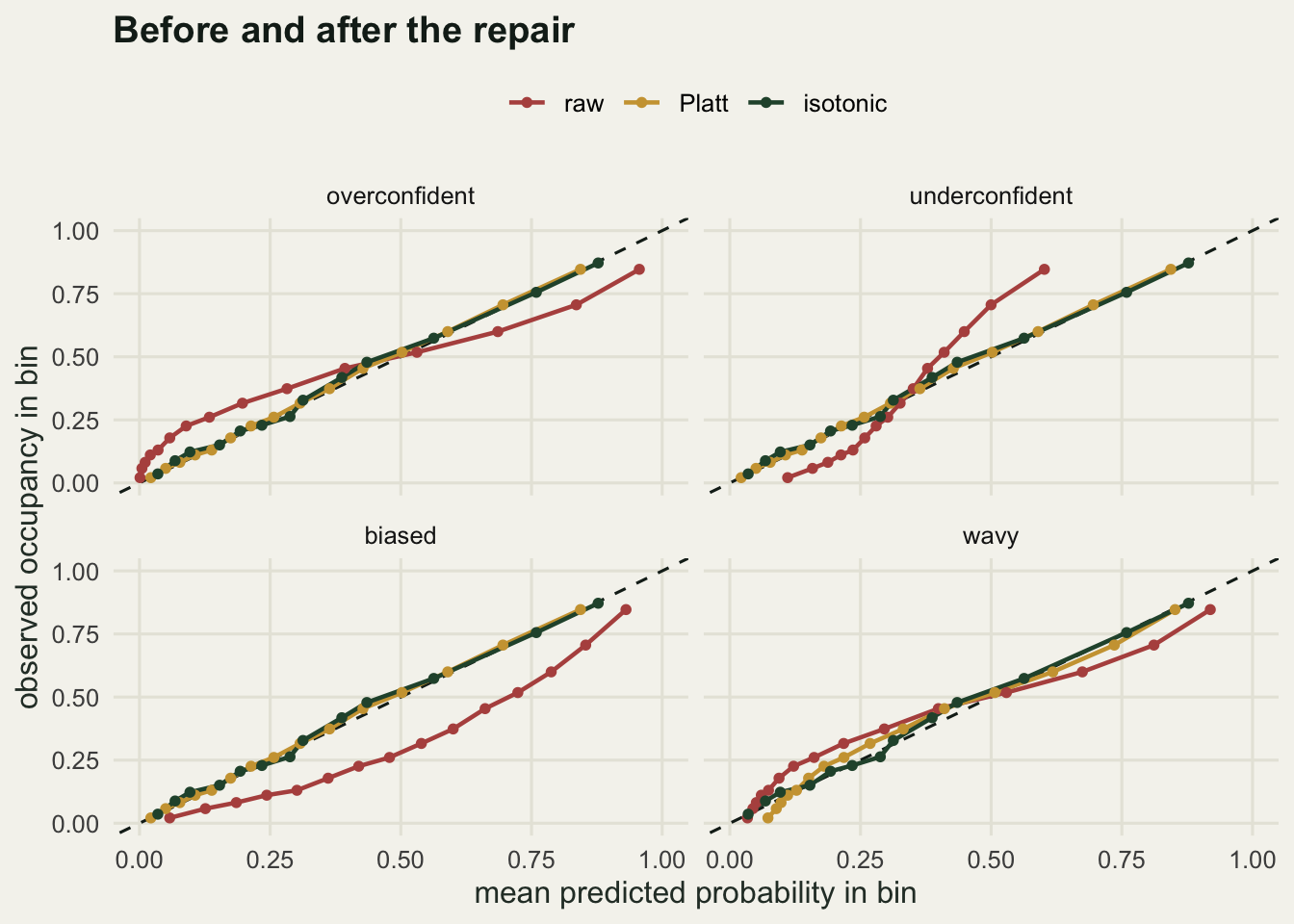

Reliability curves at 15 bins before and after calibration, for four distorted predictors. Platt scaling lands on the diagonal for the first three shapes and falls short on the wavy one; isotonic regression lands on the diagonal everywhere.

Neither repair touches the ordering in a way that could improve it. If the score is a genuinely non-monotone function of the true probability, so that some middling plots are more likely to be occupied than some high-scoring ones, no post-hoc calibration map can help: Platt scaling is monotone by construction and isotonic regression is monotone by definition. Calibration repairs the labels on the ranking, never the ranking.

What a calibrator costs, and what it buys

A calibration set is plots you did not use for fitting, which in field ecology means plots you paid for. Sweep its size from 50 to 20000, fit both calibrators on a random subset of that size, and score them on the fixed test set, averaging over 40 replicate draws. Two distortions are swept: the overconfident one, where Platt scaling is exactly right, and the wavy one, where it is not.

set.seed(20260903)
pool <- sim_plots(30000)
pool$p_fit <- predict(fit, newdata = pool, type = "response")
size_set <- c(50, 100, 200, 500, 1000, 2000, 5000, 10000, 20000)
n_rep <- 40
sweep_rows <- list()
for (nm in c("overconfident", "wavy")) {
  qpool <- warp[[nm]](pool$p_fit)
  qtest <- warp[[nm]](test$p_fit)
  raw_b <- mean((qtest - test$y)^2)
  for (ss in size_set) {
    bp <- numeric(n_rep); bo <- numeric(n_rep)
    for (r in seq_len(n_rep)) {
      idx <- sample.int(nrow(pool), ss)
      bp[r] <- mean((platt_apply(platt_fit(qpool[idx], pool$y[idx]), qtest) - test$y)^2)
      bo[r] <- mean((iso_apply(iso_fit(qpool[idx], pool$y[idx]), qtest) - test$y)^2)
    }
    sweep_rows[[length(sweep_rows) + 1]] <- data.frame(
      shape = nm, n_cal = ss, raw = raw_b, platt = mean(bp), isotonic = mean(bo))
  }
}
sweep_tab <- do.call(rbind, sweep_rows)
sweep_tab$gap <- sweep_tab$isotonic - sweep_tab$platt
cat(sprintf("replicates per calibration-set size: %d\n", n_rep))

replicates per calibration-set size: 40

print(format(sweep_tab, digits = 5), row.names = FALSE)

         shape n_cal     raw   platt isotonic         gap
 overconfident    50 0.16889 0.16822  0.17853  0.01031056
 overconfident   100 0.16889 0.16336  0.17084  0.00748212
 overconfident   200 0.16889 0.16179  0.16648  0.00469315
 overconfident   500 0.16889 0.16051  0.16311  0.00259621
 overconfident  1000 0.16889 0.16002  0.16162  0.00160116
 overconfident  2000 0.16889 0.15983  0.16085  0.00101930
 overconfident  5000 0.16889 0.15971  0.16025  0.00053572
 overconfident 10000 0.16889 0.15968  0.15995  0.00026445
 overconfident 20000 0.16889 0.15968  0.15979  0.00011510
          wavy    50 0.16477 0.16900  0.17731  0.00830487
          wavy   100 0.16477 0.16404  0.16985  0.00580537
          wavy   200 0.16477 0.16239  0.16609  0.00369948
          wavy   500 0.16477 0.16101  0.16247  0.00145790
          wavy  1000 0.16477 0.16098  0.16186  0.00087418
          wavy  2000 0.16477 0.16079  0.16091  0.00011975
          wavy  5000 0.16477 0.16062  0.16027 -0.00034809
          wavy 10000 0.16477 0.16061  0.15999 -0.00062046
          wavy 20000 0.16477 0.16058  0.15977 -0.00081133

wv <- sweep_tab[sweep_tab$shape == "wavy", ]
j <- which(wv$gap < 0)[1]
cross <- exp(approx(wv$gap[c(j - 1, j)], log(wv$n_cal[c(j - 1, j)]), xout = 0)$y)
cat(sprintf("wavy: isotonic overtakes Platt at about %.0f calibration plots\n", cross))

wavy: isotonic overtakes Platt at about 2529 calibration plots

ov <- sweep_tab[sweep_tab$shape == "overconfident", ]
cat(sprintf("overconfident: smallest gap is %.5f at %d plots, never negative\n",
            min(ov$gap), ov$n_cal[which.min(ov$gap)]))

overconfident: smallest gap is 0.00012 at 20000 plots, never negative

cat(sprintf("at 50 plots, wavy: raw %.5f, Platt %.5f, isotonic %.5f\n",
            wv$raw[1], wv$platt[1], wv$isotonic[1]))

at 50 plots, wavy: raw 0.16477, Platt 0.16900, isotonic 0.17731

The crossover exists, and it exists only where Platt scaling is misspecified. On the wavy predictor isotonic regression overtakes it at about 2529 calibration plots, and by 20000 plots it is ahead by 0.00081133 of Brier score. On the overconfident predictor there is no crossover at all: the gap shrinks steadily to 0.00012 at 20000 plots but never changes sign, because Platt scaling is the true inverse there and no amount of data lets a flexible method beat a correct one.

The small end is the part worth remembering. At 50 calibration plots the wavy predictor has a raw Brier of 0.16477, Platt scaling makes it 0.16900 and isotonic regression makes it 0.17731. Both repairs make the model worse than leaving it alone. A calibrator fitted on a handful of plots is a two-parameter or thirty-parameter model fitted to almost nothing, and it carries its own variance into every prediction.

sw_long <- rbind(
  data.frame(shape = sweep_tab$shape, n_cal = sweep_tab$n_cal,
             method = "Platt", brier = sweep_tab$platt),
  data.frame(shape = sweep_tab$shape, n_cal = sweep_tab$n_cal,
             method = "isotonic", brier = sweep_tab$isotonic))
raw_dat <- unique(sweep_tab[, c("shape", "raw")])
cross_dat <- data.frame(shape = "wavy", xc = cross)
ggplot(sw_long, aes(n_cal, brier, colour = method)) +
  geom_hline(data = raw_dat, aes(yintercept = raw), linetype = "dashed",
             colour = te_pal$ink) +
  geom_vline(data = cross_dat, aes(xintercept = xc), linetype = "dotted",
             colour = te_pal$ink) +
  geom_line(linewidth = 0.9) + geom_point(size = 1.8) +
  facet_wrap(~ shape, scales = "free_y") +
  scale_x_log10() +
  scale_colour_manual(values = c(te_pal$gold, te_pal$forest)) +
  labs(title = "What a calibration set has to be worth",
       x = "calibration plots (log scale)", y = "test Brier score", colour = NULL) +
  theme_te() + theme(legend.position = "top")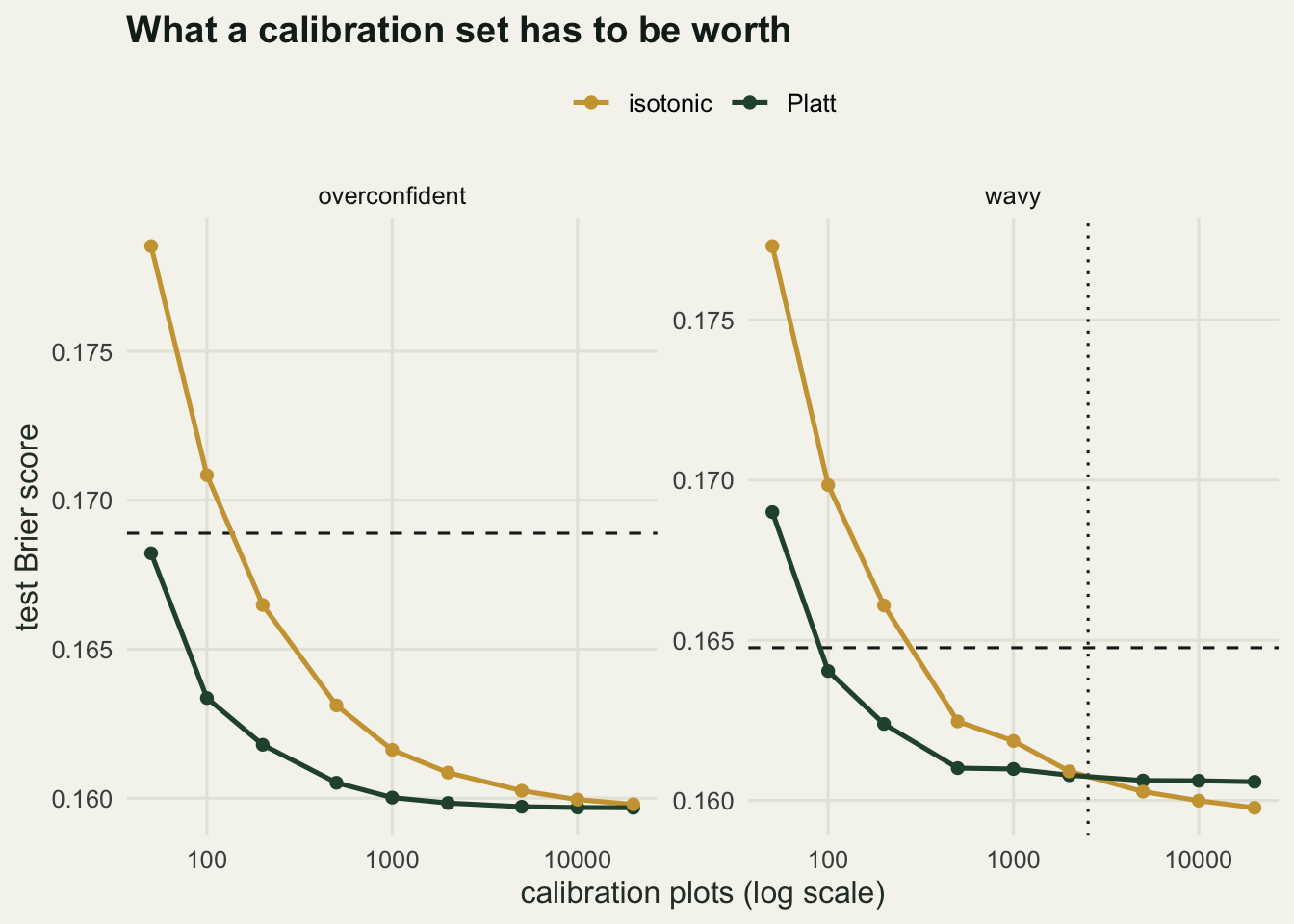

Test Brier score after calibration against the size of the calibration set, for two distortions, on free vertical scales. Dashed lines mark the uncalibrated score and the dotted line marks the measured crossover. Isotonic regression overtakes Platt scaling only where the Platt family cannot represent the distortion.

Why any of this matters is easiest to see with a decision attached. Suppose the test plots are candidate sites and the rule is to survey every plot whose predicted occupancy exceeds 0.5, while the regional estimate of occupied plots is the sum of the predictions.

thr_dec <- 0.5
q_cal_m  <- warp$calibrated(test$p_fit)
q_und_m  <- warp$underconfident(test$p_fit)
q_bias_m <- warp$biased(test$p_fit)
dec_tab <- data.frame(
  model = c("calibrated", "underconfident", "biased"),
  expected_occupied = c(sum(q_cal_m), sum(q_und_m), sum(q_bias_m)),
  plots_flagged = c(sum(q_cal_m >= thr_dec), sum(q_und_m >= thr_dec),
                    sum(q_bias_m >= thr_dec)),
  occupied_found = c(sum(test$y[q_cal_m >= thr_dec]), sum(test$y[q_und_m >= thr_dec]),
                     sum(test$y[q_bias_m >= thr_dec])),
  auc = c(auc_rank(q_cal_m, test$y), auc_rank(q_und_m, test$y),
          auc_rank(q_bias_m, test$y)))
cat(sprintf("decision threshold %.2f, truly occupied test plots %d\n",
            thr_dec, sum(test$y)))

decision threshold 0.50, truly occupied test plots 13016

print(format(dec_tab, digits = 6), row.names = FALSE)

          model expected_occupied plots_flagged occupied_found      auc
     calibrated           13147.2          9894           6731 0.812198
 underconfident           12694.6          3951           3217 0.812198
         biased           19384.6         19054          10279 0.812198

cat(sprintf("flagged ratio, biased over underconfident: %.2f\n",
            dec_tab$plots_flagged[3] / dec_tab$plots_flagged[2]))

flagged ratio, biased over underconfident: 4.82

cat(sprintf("expected-count error: underconfident %.0f, biased %+.0f plots\n",
            dec_tab$expected_occupied[2] - sum(test$y),
            dec_tab$expected_occupied[3] - sum(test$y)))

expected-count error: underconfident -321, biased +6369 plots

The underconfident model flags 3951 plots for survey and the biased one flags 19054, a ratio of 4.82, from identical rankings and an identical AUC of 0.812198. The calibrated model flags 9894 and finds 6731 occupied plots among them. As a regional estimate the biased model predicts 6369 occupied plots more than the 13016 that exist, an overstatement of nearly half. Which of these three you deploy is a decision about survey effort and about a published population figure, and the diagnostic normally used to choose between models rates them identically.

What calibration cannot tell you

Calibration is a joint property of a model and a population, never a property of the model alone. Move the model to a region with different occupancy and it is no longer calibrated there, whatever it did at home. Two versions of that move are worth separating, because only one of them has a cheap fix. Below, a region with the same covariate response but lower occupancy, and a region where the response to deadwood is shallower. In each, half the plots fit the correction and the other half measure it.

set.seed(20260904)
sim_region <- function(nn, b0, b1) {
  deadwood <- rnorm(nn); openness <- rnorm(nn)
  pt <- plogis(b0 + b1 * deadwood + 0.7 * openness)
  data.frame(deadwood = deadwood, openness = openness,
             p_true = pt, y = rbinom(nn, 1, pt))
}
n_region <- 20000
regions <- list("lower occupancy only" = sim_region(n_region, -2.4, 1.3),
                "shallower response"   = sim_region(n_region, -1.0, 0.6))
for (nm in names(regions)) {
  dd <- regions[[nm]]
  dd$p_fit <- predict(fit, newdata = dd, type = "response")
  half <- seq_len(n_region) %% 2 == 0
  zz <- lg(pmin(pmax(dd$p_fit[half], 1e-6), 1 - 1e-6))
  a_hat <- unname(coef(glm(dd$y[half] ~ offset(zz), family = binomial)))
  q_int <- plogis(a_hat + lg(pmin(pmax(dd$p_fit[!half], 1e-6), 1 - 1e-6)))
  bcf <- platt_fit(dd$p_fit[half], dd$y[half])
  q_pl <- platt_apply(bcf, dd$p_fit[!half])
  yv <- dd$y[!half]
  cat(sprintf("%s: occupancy %.4f, mean prediction %.4f\n",
              nm, mean(dd$y), mean(dd$p_fit)))
  cat(sprintf("   reliability  raw %.5f  intercept only %.5f  full Platt %.5f\n",
              rel_comp(dd$p_fit[!half], yv), rel_comp(q_int, yv), rel_comp(q_pl, yv)))
  cat(sprintf("   Brier        raw %.5f  intercept only %.5f  full Platt %.5f\n",
              mean((dd$p_fit[!half] - yv)^2), mean((q_int - yv)^2), mean((q_pl - yv)^2)))
  cat(sprintf("   intercept shift %.4f, Platt slope %.4f\n", a_hat, bcf[2]))
}

lower occupancy only: occupancy 0.1447, mean prediction 0.3293
   reliability  raw 0.04384  intercept only 0.00012  full Platt 0.00008
   Brier        raw 0.14072  intercept only 0.09666  full Platt 0.09661
   intercept shift -1.4055, Platt slope 1.0516
shallower response: occupancy 0.2993, mean prediction 0.3267
   reliability  raw 0.00874  intercept only 0.00675  full Platt 0.00017
   Brier        raw 0.19622  intercept only 0.19423  full Platt 0.18771
   intercept shift -0.1888, Platt slope 0.5916

Where only the occupancy rate has changed, an intercept shift is the whole repair. The model predicts a mean of 0.3293 into a region where occupancy is 0.1447, reliability is 0.04384, and adding -1.4055 to every logit brings it to 0.00012. Fitting the slope as well adds almost nothing: 0.00008, and the estimated slope is 1.0516, near enough to one. Where the response itself is shallower, the intercept alone gets reliability from 0.00874 to 0.00675 and stops, while the two-parameter fit reaches 0.00017 with a slope of 0.5916. The rule of thumb is that an intercept correction buys you a base rate and nothing else, and if you cannot tell which kind of shift you are facing, you need the held-out plots either way.

The second limit is sharper. Every number above comes from data the model never saw, and that is not a stylistic preference. A logistic model fitted by maximum likelihood with an intercept satisfies the score equation that the fitted probabilities sum to the observed successes, so its calibration on its own training data is guaranteed, not measured. Fitting 42 predictors to 400 plots, of which 40 predictors are pure noise, shows what that guarantee is worth.

set.seed(20260905)
n_small <- 400; n_noise <- 40
mk_small <- function(nn) {
  xx <- matrix(rnorm(nn * (2 + n_noise)), nn, 2 + n_noise)
  dfr <- as.data.frame(xx)
  dfr$y <- rbinom(nn, 1, plogis(-1.0 + 1.3 * xx[, 1] + 0.7 * xx[, 2]))
  dfr
}
small_tr <- mk_small(n_small)
small_te <- mk_small(20000)
fit_big <- suppressWarnings(glm(y ~ ., data = small_tr, family = binomial))
p_in  <- fitted(fit_big)
p_out <- predict(fit_big, newdata = small_te, type = "response")
null_in <- replicate(200, rel_comp(p_in, rbinom(n_small, 1, p_in)))
cat(sprintf("predictors %d (2 real, %d noise), training plots %d\n",
            2 + n_noise, n_noise, n_small))

predictors 42 (2 real, 40 noise), training plots 400

cat(sprintf("training: Brier %.5f, reliability %.5f, null median %.5f, sum(y - p) %.2e\n",
            mean((p_in - small_tr$y)^2), rel_comp(p_in, small_tr$y),
            median(null_in), sum(small_tr$y - p_in)))

training: Brier 0.13409, reliability 0.00231, null median 0.00285, sum(y - p) -3.88e-13

cat(sprintf("held out: Brier %.5f, reliability %.5f\n",
            mean((p_out - small_te$y)^2), rel_comp(p_out, small_te$y)))

held out: Brier 0.19697, reliability 0.01375

On its own training plots the model has a reliability of 0.00231, below the null median of 0.00285 that a perfectly calibrated forecaster would produce at that sample size, and the residuals sum to -3.83e-13. It looks flawless. On fresh plots the reliability is 0.01375 and the Brier score goes from 0.13409 to 0.19697. A reliability diagram drawn on training data is a picture of an algebraic identity. It cannot fail, so it cannot inform.

The last thing none of this covers: calibration says nothing about whether the covariates are the right ones, or whether the plots were chosen in a way that represents the region. A perfectly calibrated model of a biased sample is perfectly calibrated on that bias.

Where to go next

Calibrated probabilities are an input, not an answer. What turns them into a decision is a statement about what a missed occupied plot costs relative to a wasted survey visit, and the threshold that follows from those two numbers is almost never 0.5. The next tutorial in this cluster works through choosing a decision threshold from costs, including what happens to that threshold when the prevalence changes and when the cost ratio is only known to within a factor of two.

References

Murphy AH 1973 Journal of Applied Meteorology 12(4):595-600 (10.1175/1520-0450(1973)012<0595:ANVPOT>2.0.CO;2)

Niculescu-Mizil A, Caruana R 2005 Proceedings of the 22nd International Conference on Machine Learning:625-632 (10.1145/1102351.1102430)

Zadrozny B, Elkan C 2002 Proceedings of the 8th ACM SIGKDD International Conference on Knowledge Discovery and Data Mining:694-699 (10.1145/775047.775151)

Van Calster B, McLernon DJ, van Smeden M, Wynants L, Steyerberg EW 2019 BMC Medicine 17:230 (10.1186/s12916-019-1466-7)

Gneiting T, Raftery AE 2007 Journal of the American Statistical Association 102(477):359-378 (10.1198/016214506000001437)

Related tutorials

• Class imbalance in species presence models
• Data leakage in ecological model validation
• Choosing a decision threshold from costs
• The CRPS and the Brier score