---
title: "The CRPS and the Brier score"
description: "Two proper scores for ecological forecasts: the Brier score for presence, the CRPS for abundance, built from scratch in R with the identities linking them."
date: "2026-06-25 09:00"
categories: [R, forecasting, model evaluation, ecology tutorial]
date-modified: "2026-10-01"
image: thumbnail.png
image-alt: "A forecast cumulative distribution function and the step function at the outcome, with the gap between them shaded; the CRPS integrates the square of that gap."
---
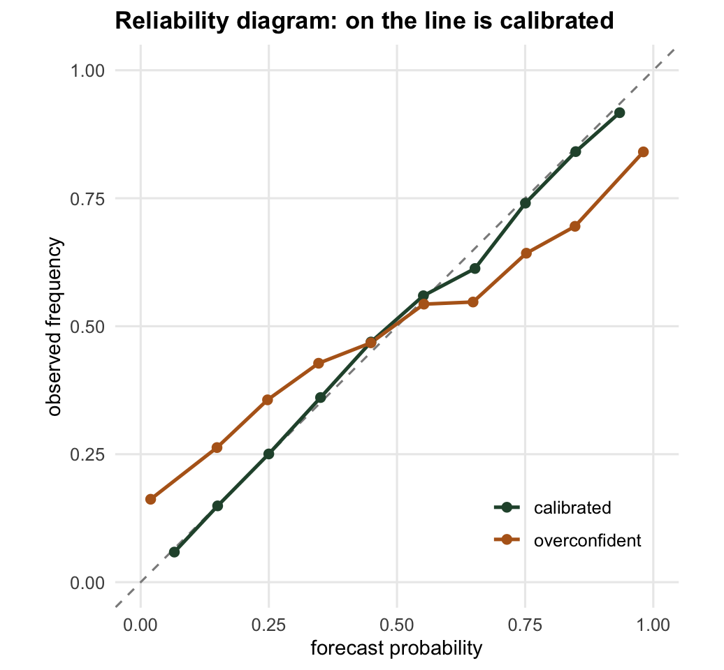
*Corrected 1 October 2026: the text description of the reliability diagram called the overconfident curve S-shaped; it now describes the flatter, nearly straight line the code draws.*
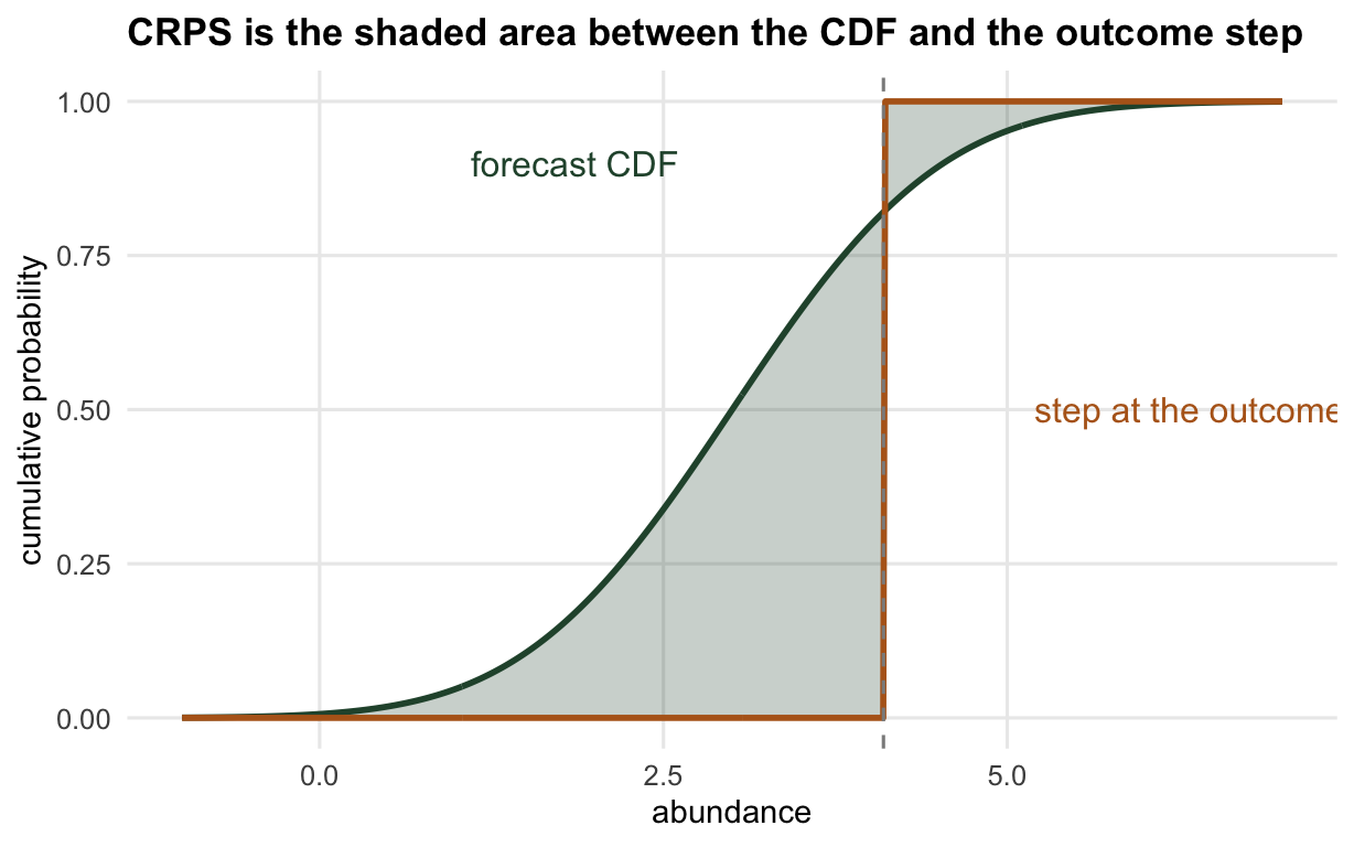
*Corrected 27 September 2026: the figure caption and title said the CRPS is the shaded area between the forecast CDF and the outcome step; the CRPS integrates the squared height of that gap, so it is smaller than the shaded area, and the labels now say so.*
The [previous post](../scoring-ecological-forecasts/) argued that a forecast should be scored as a distribution, and that the rule should be proper. The log score qualifies, but it is brittle: put zero probability on something that happens and the score is infinite, which is a real hazard for the count and presence data ecologists work with. Two scores avoid that and dominate practice. The **Brier score** grades a presence or absence forecast. The **continuous ranked probability score** (CRPS) grades a forecast of a continuous quantity like abundance or a date. Both are proper, neither can be infinite for a forecast with a finite mean, and they are the same idea viewed at two resolutions. Only the Brier score is bounded, living in the unit interval; the CRPS carries the units of the outcome and is as large as the outcome can be wrong.
## The Brier score for presence and absence
A species distribution model predicts a probability of presence at each site. The outcome is 0 or 1. The Brier score is the mean squared distance between the two: identical in form to mean squared error, but applied to a probability.
```{r setup}
#| echo: false
#| message: false
#| warning: false
suppressMessages(library(ggplot2))
te_canvas <- theme(plot.background = element_rect(fill = "#f5f4ee", colour = NA),
panel.background = element_rect(fill = "#f5f4ee", colour = NA))
col_main <- "#275139"; col_acc <- "#B5651D"; col_mut <- "#8C8C8C"
base_th <- theme_minimal(base_size = 12) + te_canvas +
theme(panel.grid.minor = element_blank(),
plot.title = element_text(face = "bold", size = 13),
axis.title = element_text(size = 11))
```
```{r brier}
set.seed(202)
n <- 4000
p_true <- plogis(rnorm(n, 0, 1.3))   # true presence probabilities across sites
y <- rbinom(n, 1, p_true)            # realised presence/absence
p_fore <- p_true                     # a well-calibrated forecast

brier <- function(p, y) mean((p - y)^2)
BS <- brier(p_fore, y)
BS
```
The calibrated forecast scores `r sprintf("%.3f", BS)`. Lower is better; a perfect deterministic forecast scores 0, and a forecast that says 0.5 everywhere scores 0.25. The Brier score is proper (Brier 1950): the site-by-site expected score is minimised by reporting the true probability.
Its real value is that it splits into interpretable pieces. Murphy's decomposition (1973) bins the forecasts and writes the score as reliability minus resolution plus uncertainty: reliability measures how far each bin's forecast probability sits from the frequency observed in that bin (calibration), resolution measures how much the bins separate high-risk from low-risk sites (discrimination), and uncertainty is the base rate variance you cannot avoid.
```{r brier-decomp}
K <- 10
bin <- cut(p_fore, breaks = seq(0, 1, length.out = K + 1), include.lowest = TRUE)
obar <- mean(y)
rel <- res <- 0
for (b in levels(bin)) {
  idx <- bin == b; nk <- sum(idx); if (nk == 0) next
  pbar_k <- mean(p_fore[idx]); obar_k <- mean(y[idx])
  rel <- rel + nk / n * (pbar_k - obar_k)^2      # reliability (calibration)
  res <- res + nk / n * (obar_k - obar)^2        # resolution (discrimination)
}
unc <- obar * (1 - obar)                          # uncertainty (base rate)
c(reliability = rel, resolution = res, uncertainty = unc, sum = rel - res + unc,
  binned_brier = mean((ave(p_fore, bin) - y)^2))
```
Reliability is near zero (`r sprintf("%.4f", rel)`), because the forecast is calibrated; resolution is `r sprintf("%.3f", res)`, the part the forecast earns by separating sites; uncertainty is `r sprintf("%.3f", unc)`. They reconstruct the binned Brier score exactly: `sum` and `binned_brier` agree to machine precision, and the binned score sits at `r sprintf("%.4f", mean((ave(p_fore, bin) - y)^2))` against the raw `r sprintf("%.4f", BS)` because binning discards the spread of forecasts inside each bin. That is why the decomposition is an exact accounting of where the binned score comes from, and only an approximation to the raw one. Push the same forecast toward overconfidence (stretch the probabilities toward 0 and 1) and the Brier score gets worse:
```{r brier-over}
p_over <- pmin(pmax(1.6 * (p_fore - 0.5) + 0.5, 0), 1)   # sharpen toward the extremes
c(calibrated = brier(p_fore, y), overconfident = brier(p_over, y))
```
The overconfident forecast scores `r sprintf("%.3f", brier(p_over, y))` against `r sprintf("%.3f", brier(p_fore, y))`; the proper score sees through the false precision.
```{r fig-reliability}
#| echo: false
#| fig-cap: "Reliability diagram. Points on the diagonal are calibrated; the overconfident forecast sits above the line at low probabilities and below it at high ones."
#| fig-alt: "Reliability diagram with observed frequency against forecast probability. The calibrated curve tracks the diagonal; the overconfident curve is a flatter, nearly straight line that crosses the diagonal in the middle."
#| fig-width: 5.4
#| fig-height: 5.0
relib <- function(p, y, K = 10) { b <- cut(p, seq(0, 1, length.out = K + 1), include.lowest = TRUE)
data.frame(pbar = tapply(p, b, mean), obar = tapply(y, b, mean)) }
d2b <- rbind(cbind(relib(p_fore, y), who = "calibrated"),
cbind(relib(p_over, y), who = "overconfident"))
ggplot(d2b, aes(pbar, obar, colour = who)) +
geom_abline(slope = 1, intercept = 0, linetype = "dashed", colour = col_mut) +
geom_line(linewidth = 0.9) + geom_point(size = 2) +
scale_colour_manual(values = c(col_main, col_acc), name = NULL) +
coord_equal(xlim = c(0, 1), ylim = c(0, 1)) +
labs(title = "Reliability diagram: on the line is calibrated",
x = "forecast probability", y = "observed frequency") +
base_th + theme(legend.position = "inside", legend.position.inside = c(0.8, 0.15))
```
## The CRPS for a continuous outcome
Abundance and dates are not binary, so the Brier score does not apply directly. The CRPS is the generalisation. Its definition is geometric: take the forecast cumulative distribution function, take the step function that jumps from 0 to 1 at the outcome, and integrate the squared gap between them over the whole line (Matheson and Winkler 1976). A forecast concentrated near the truth leaves little gap and scores low.
```{r fig-crps-area}
#| echo: false
#| fig-cap: "The shaded gap lies between the forecast CDF and the orange step function at the outcome. The CRPS integrates the squared height of this gap, so it is smaller than the shaded area itself."
#| fig-alt: "A smooth S-shaped forecast cumulative distribution function and an orange step function jumping to one at the outcome, with the region between them shaded green."
#| fig-width: 6.4
#| fig-height: 4.0
mu_f <- 3.0; sig_f <- 1.2; y_val <- 4.1
xg <- seq(-1, 7, length.out = 500)
Fx <- pnorm(xg, mu_f, sig_f); step <- as.numeric(xg >= y_val)
ggplot(data.frame(x = xg, Fx = Fx, step = step), aes(x)) +
geom_ribbon(aes(ymin = pmin(Fx, step), ymax = pmax(Fx, step)), fill = col_main, alpha = 0.25) +
geom_line(aes(y = Fx), colour = col_main, linewidth = 1) +
geom_line(aes(y = step), colour = col_acc, linewidth = 1) +
geom_vline(xintercept = y_val, linetype = "dashed", colour = col_mut) +
annotate("text", x = 1.1, y = 0.9, label = "forecast CDF", colour = col_main, hjust = 0) +
annotate("text", x = 5.2, y = 0.5, label = "step at the outcome", colour = col_acc, hjust = 0) +
labs(title = "CRPS integrates the squared gap between the CDF and the step",
x = "abundance", y = "cumulative probability") + base_th
```
For a Gaussian predictive there is a closed form, so you never have to integrate by hand:
```{r crps-forms}
crps_norm <- function(mu, sigma, y) {          # closed form for a Normal forecast
  z <- (y - mu) / sigma
  sigma * (z * (2 * pnorm(z) - 1) + 2 * dnorm(z) - 1 / sqrt(pi))
}
mu_f <- 3.0; sig_f <- 1.2; y_val <- 4.1
cf <- crps_norm(mu_f, sig_f, y_val)

# check it against the definition by direct numerical integration
xg2 <- seq(-60, 60, length.out = 2e6)
nd <- sum((pnorm(xg2, mu_f, sig_f) - as.numeric(xg2 >= y_val))^2) * (xg2[2] - xg2[1])
c(closed_form = cf, numerical = nd)
```
The closed form (`r sprintf("%.4f", cf)`) matches the brute-force integral of the definition to four decimals, the rest being the grid spacing of the numerical integral, which confirms the formula. Two identities make the CRPS easy to reason about. First, a forecast that is a single point (no spread) has a CRPS equal to the absolute error, so the CRPS is the natural generalisation of mean absolute error to distributions:
```{r crps-pointmass}
c(crps_pointmass = crps_norm(mu_f, 1e-4, y_val), abs_error = abs(y_val - mu_f))
```
As the spread shrinks to nothing the CRPS collapses to `r sprintf("%.3f", abs(y_val - mu_f))`, the plain absolute error. Second, when you only have an ensemble of draws rather than a formula, the CRPS has a fair estimator built from pairwise distances: the mean distance from the draws to the outcome, minus half the mean distance among the draws themselves.
```{r crps-ensemble}
crps_fair <- function(x, y) { m <- length(x)
  mean(abs(x - y)) - 0.5 * sum(outer(x, x, function(a, b) abs(a - b))) / (m * (m - 1)) }
set.seed(2025)
ens <- rnorm(10000, mu_f, sig_f)
c(ensemble = crps_fair(ens, y_val), closed_form = cf)
```
The ensemble estimate (`r sprintf("%.4f", crps_fair(ens, y_val))`) lands on the closed form, so the same score works whether your forecast is a fitted distribution or a bag of simulations from a state-space model.
## The two scores are one idea
The CRPS is not a separate invention; it is the Brier score integrated over every possible threshold. Fix a threshold, ask the binary question "will the outcome exceed it?", and the Brier score of that yes/no forecast is the squared gap between the CDF and the step at that point. Sum those Brier scores across all thresholds and you have rebuilt the CRPS.
```{r crps-brier-link}
tg <- seq(-60, 60, length.out = 2e6)
crps_via_brier <- sum((pnorm(tg, mu_f, sig_f) - as.numeric(y_val <= tg))^2) * (tg[2] - tg[1])
c(via_threshold_brier = crps_via_brier, closed_form = cf)
```
The threshold-by-threshold Brier integral (`r sprintf("%.4f", crps_via_brier)`) equals the CRPS. So the Brier score is the CRPS at one resolution, and the CRPS is the Brier score at all of them. Learn one and you have the other.
## Where to go next
A CRPS of `r sprintf("%.2f", cf)` means nothing on its own; it is not good or bad until you compare it to something. The next post is about that comparison: skill scores, the baselines you measure against, and the uncomfortable fact that the same forecast can be skilful against one baseline and useless against another.
## References
Brier GW 1950. Monthly Weather Review 78(1):1-3 (10.1175/1520-0493(1950)078<0001:VOFEIT>2.0.CO;2)
Matheson JE, Winkler RL 1976. Management Science 22(10):1087-1096 (10.1287/mnsc.22.10.1087)
Murphy AH 1973. Journal of Applied Meteorology 12(4):595-600 (10.1175/1520-0450(1973)012<0595:ANVPOT>2.0.CO;2)
Gneiting T, Raftery AE 2007. Journal of the American Statistical Association 102(477):359-378 (10.1198/016214506000001437)
## Related tutorials
- [Scoring ecological forecasts](../scoring-ecological-forecasts/)
- [Forecast skill and the baseline](../forecast-skill-and-the-baseline/)
- [Checking a forecast evaluation](../checking-a-forecast-evaluation/)
- [Calibrating predicted probabilities in R](../probability-calibration-for-classifiers/)