---
title: "Forecast skill and the baseline"
description: "A raw forecast score means nothing without a baseline. In R, the same ecological forecast is skilful against one reference and useless against another."
date: "2026-06-25 10:00"
date-modified: "2026-10-07"
categories: [R, forecasting, model evaluation, ecology tutorial]
image: thumbnail.png
image-alt: "Two skill-score curves against series autocorrelation, one for a climatology baseline and one for persistence, crossing zero at different points."
---
*Corrected 7 October 2026: a code comment called the model under-damped, the opposite of what the text says; it now says the model has too little memory. The closing advice said a change of reference can reverse the ordering of two forecasts; it now says that a shared reference ranks them as their raw scores do, and a reversal needs the two to be scored against different references.*
The [CRPS post](../the-crps-and-brier-score/) ended on a loose thread: a score of 0.66 is a number with no meaning until you compare it to something. That comparison is the **skill score**, and it turns a raw score into a statement of the form "my forecast beats a simple baseline by this much". The catch, and the whole point of this post, is that the baseline is a choice, and the same forecast can look skilful or worthless depending on which baseline you pick. This is not a technicality; it is the most common way an ecological forecast is oversold.
## Skill is a comparison, not a property
A skill score rescales your score against a reference forecast: one minus your score divided by the reference's score. Positive means you beat the reference; zero means you tied it; negative means the reference was better. Two references are standard in ecology (Dietze et al. 2018; Harris et al. 2018). **Climatology** predicts next year from the long-run distribution: next year looks like a random past year. **Persistence** predicts next year from this year: next year looks like the last observation. They are easy to beat in different situations, and that is where the trouble starts.
```{r setup}
#| message: false
#| warning: false
#| code-fold: true
#| code-summary: "Setup: packages, colours and plot theme"
suppressMessages(library(ggplot2))
te_canvas <- theme(plot.background  = element_rect(fill = "#f5f4ee", colour = NA),
                   panel.background = element_rect(fill = "#f5f4ee", colour = NA))
col_main <- "#275139"; col_acc <- "#B5651D"; col_mut <- "#8C8C8C"
base_th <- theme_minimal(base_size = 12) + te_canvas +
  theme(panel.grid.minor = element_blank(),
        plot.title = element_text(face = "bold", size = 13),
        axis.title = element_text(size = 11))
crps_norm <- function(mu, sigma, y) { z <- (y - mu) / sigma
  sigma * (z * (2 * pnorm(z) - 1) + 2 * dnorm(z) - 1 / sqrt(pi)) }
```
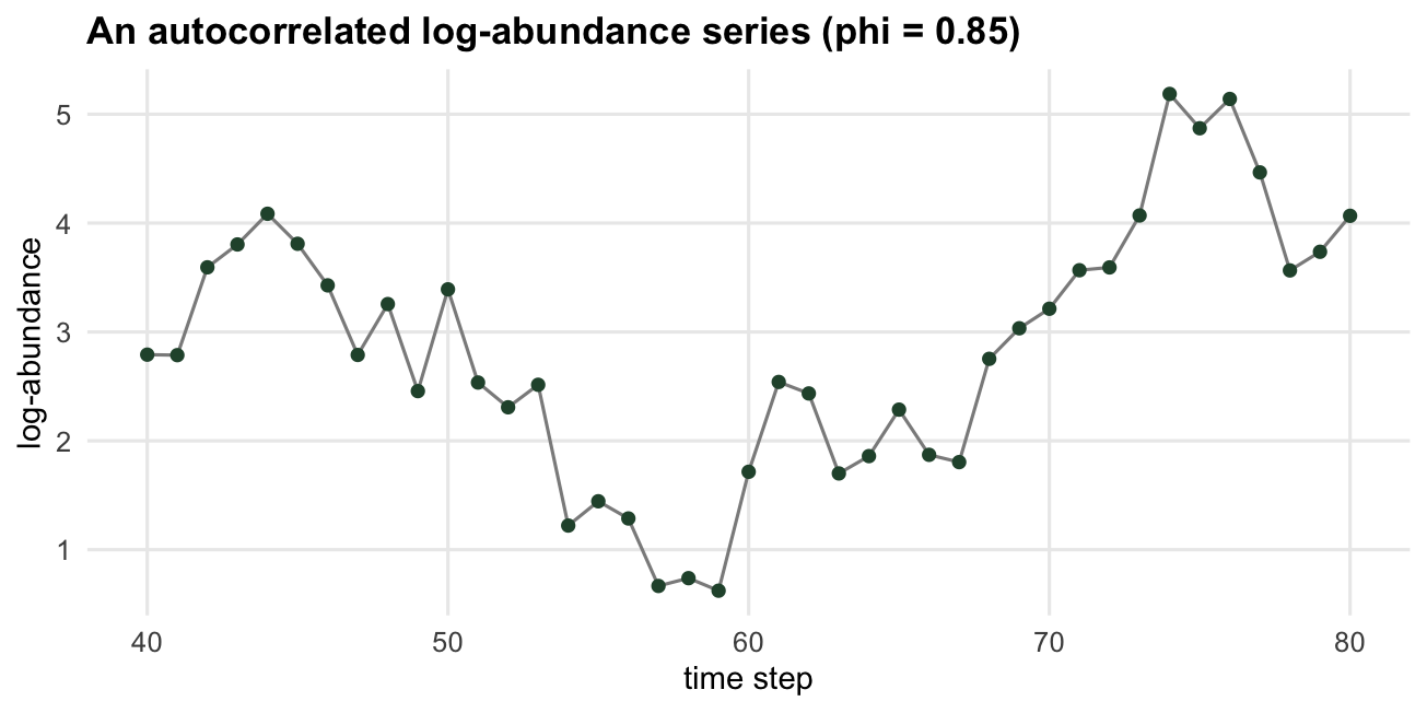
Take a population whose log-abundance follows an order-one autoregressive process: each year reverts partway toward a long-run mean, with environmental noise on top. The strength of that year-to-year memory is the autocorrelation, and it controls which baseline is hard to beat. When memory is strong, this year is a great guess for next year, so persistence is tough and climatology is weak. When memory is weak, the reverse holds.
```{r series}
simulate_series <- function(phi, sp, m0 = 3, n = 6000, seed = 303) {
  set.seed(seed); x <- numeric(n); x[1] <- m0
  for (t in 2:n) x[t] <- m0 + phi * (x[t - 1] - m0) + rnorm(1, 0, sp)
  x
}
x <- simulate_series(phi = 0.85, sp = 0.5)   # strongly autocorrelated series
```
```{r fig-series}
#| echo: false
#| fig-cap: "A log-abundance series with strong year-to-year memory (autocorrelation 0.85). Here last year is a good guess for next year."
#| fig-alt: "A time series of log-abundance over about forty steps, wandering smoothly around a central level with gradual drifts rather than sharp jumps."
#| fig-width: 6.8
#| fig-height: 3.4
win <- 40:80
ggplot(data.frame(t = win, obs = x[win]), aes(t, obs)) +
geom_line(colour = col_mut) + geom_point(colour = col_main, size = 1.6) +
labs(title = "An autocorrelated log-abundance series (phi = 0.85)",
x = "time step", y = "log-abundance") + base_th
```
## The same forecast, opposite verdicts
Now fix one forecast and score it against both baselines. The forecast is a reasonable but imperfect model: it uses the autocorrelation, but underestimates it (it assumes weaker memory than the series really has). Its CRPS, and the two baselines' CRPS, are computed on the same series.
```{r score-forecasts}
score_forecasts <- function(phi_true, sp = 0.5, phi_model = 0.4, m0 = 3) {
  x <- simulate_series(phi_true, sp, m0); n <- length(x); idx <- 2:n
  smarg <- sp / sqrt(1 - phi_true^2)                         # stationary marginal sd
  mu_m <- m0 + phi_model * (x[idx - 1] - m0)                 # the model (too little memory)
  s_m  <- smarg * sqrt(1 - phi_model^2)
  sdiff <- sp * sqrt(2 / (1 + phi_true))                     # sd of the year-to-year change
  y <- x[idx]
  c(model = mean(crps_norm(mu_m, s_m, y)),
    clim  = mean(crps_norm(rep(m0, length(idx)), rep(smarg, length(idx)), y)),   # climatology
    pers  = mean(crps_norm(x[idx - 1], rep(sdiff, length(idx)), y)))             # persistence
}
skill <- function(s_fore, s_ref) 1 - s_fore / s_ref

S <- score_forecasts(phi_true = 0.85)
c(S, skill_vs_clim = skill(S["model"], S["clim"]),
     skill_vs_pers = skill(S["model"], S["pers"]))
```
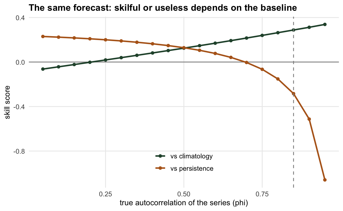
Read the two skill numbers. Against climatology the model has skill `r sprintf("%+.3f", skill(S["model"], S["clim"]))`: clearly positive, a useful forecast. Against persistence the skill is `r sprintf("%+.3f", skill(S["model"], S["pers"]))`: negative, worse than simply repeating last year's value. This is one forecast, one series, one CRPS. The verdict flipped because the reference changed. A paper reporting only the climatology comparison would call this model skilful; a reviewer who asked for persistence would call it a failure. Both are looking at the same forecast.
The mechanism is not subtle once you sweep the autocorrelation. Climatology is hard to beat when there is little memory to exploit; persistence is hard to beat when there is a lot. The model sits in between, so its skill against each baseline crosses zero at a different point, and there is only a window of autocorrelation where it beats both.
```{r skill-sweep}
phis <- seq(0.05, 0.95, by = 0.05)
sk <- t(sapply(phis, function(ph) {
  s <- score_forecasts(ph)
  c(vs_clim = skill(s["model"], s["clim"]), vs_pers = skill(s["model"], s["pers"]))
}))
head(round(sk, 3))
```
```{r fig-skill}
#| echo: false
#| fig-cap: "Skill of one forecast against two baselines, across series autocorrelation. Below about 0.2 it loses to climatology; above about 0.7 it loses to persistence."
#| fig-alt: "Two curves of skill score against autocorrelation. The climatology curve rises steadily from slightly negative to clearly positive; the persistence curve falls from positive to strongly negative; they cross zero at different autocorrelations."
#| fig-width: 6.8
#| fig-height: 4.2
d3 <- data.frame(phi = rep(phis, 2), skill = c(sk[, 1], sk[, 2]),
baseline = rep(c("vs climatology", "vs persistence"), each = length(phis)))
ggplot(d3, aes(phi, skill, colour = baseline)) +
geom_hline(yintercept = 0, colour = col_mut) +
geom_line(linewidth = 1) + geom_point(size = 1.6) +
geom_vline(xintercept = 0.85, linetype = "dashed", colour = col_mut) +
scale_colour_manual(values = c(col_main, col_acc), name = NULL) +
labs(title = "The same forecast: skilful or useless depends on the baseline",
x = "true autocorrelation of the series (phi)", y = "skill score") +
base_th + theme(legend.position = "inside", legend.position.inside = c(0.5, 0.15))
```
The climatology curve crosses zero near 0.2 and climbs steadily after it; the persistence curve crosses zero near 0.7 and falls ever more steeply after it. At the dashed line (0.85) they land on opposite sides of zero, which is the split we just computed.
## The honest limit
Skill is not accuracy. It is a ranking relative to a reference, and a good skill score against a weak reference says more about the reference than about your model. The practical rules follow directly. Report skill against a baseline that is genuinely hard for your system, not one chosen because you beat it: for a strongly autocorrelated population that means persistence, not climatology. Report the baseline's own score too, so a reader can see whether you cleared a low bar or a high one. And when you compare two forecasts, hold the baseline fixed: scored against one shared reference, two forecasts rank by skill exactly as they rank by raw score, but scoring one against climatology and the other against persistence can reverse that ordering without either forecast changing at all.
## Where to go next
The window where a forecast beats every reasonable baseline is real, but it can still hide problems: a forecast can post a good score while being badly calibrated, or the score difference between two models can be noise. The last post in this cluster is the checking step, three diagnostics that catch the ways a forecast evaluation misleads even when the headline number looks fine.
## References
Dietze MC, Fox A, Beck-Johnson LM, et al. 2018. Proceedings of the National Academy of Sciences 115(7):1424-1432 (10.1073/pnas.1710231115)
Harris DJ, Taylor SD, White EP 2018. PeerJ 6:e4278 (10.7717/peerj.4278)
Dietze MC 2017. Ecological Forecasting. Princeton University Press (ISBN 978-1-4008-8545-9)
## Related tutorials
- [The CRPS and the Brier score](../the-crps-and-brier-score/)
- [Checking a forecast evaluation](../checking-a-forecast-evaluation/)
- [Validating an SDM against a resurvey](../validating-an-sdm-against-a-resurvey/)
- [Smoothing a series before testing a forecast](../smoothing-before-a-forecast-test/)