Validating an SDM against a resurvey

A resurvey tests an SDM on change, yet the old map can beat it and even the true niche misses many extirpations. How species turnover sets the verdict, in R.

A county flora was mapped square by square in the early 1990s, and the same squares were mapped again last year. In between, someone fitted a distribution model to the first atlas, projected it onto the warmer climate of the second, and the second atlas is now the test the model was waiting for. Temporal validation of this kind is the check reviewers ask for, because it is the only one where the model is scored on a period it never saw. The scores come back, and they are disappointing in a particular way. The projected map agrees with the new atlas reasonably well where nothing changed, and badly where something did: many of the squares that lost the plant were not squares the model had written off. Rapacciuolo and colleagues (2012) found that pattern for British plants, birds and butterflies, and Auffret, Nenzen and Polaina (2024) found it again for plants in Sweden projected over most of a century, where the models foresaw fewer than a third of each species’ extirpations on average.

Two questions sit behind that disappointment, and neither is about the choice of algorithm. The first is what a perfect model would have scored. A square can lose a plant for no reason a climate layer could know about, and a model that knew the true suitability of every square would still miss those losses. The second is what the model is being compared against. Forecast skill and the baseline makes the general point on an abundance series: a score means nothing without a reference, and for a population with strong memory the hard reference is persistence, next year looks like this year. That post scores a continuous forecast on a time series with the CRPS; this one does not re-teach skill scores. It takes the persistence principle to a binary map, where persistence means handing in the first atlas unchanged as the forecast for the second, and asks when that old map beats the model.

The answer depends on a rate that one survey cannot see. How fast squares change hands is the colonisation and extinction machinery of dynamic occupancy: colonisation and extinction, and occupancy turnover and equilibrium derives the equilibrium and the turnover from those two rates. Here the same two rates drive a species on a climate gradient, and the post measures what they do to the verdict of a resurvey. The resurvey in checking a range shift analysis is a different object: there it is a source of effort bias in an edge estimate, and here every square is visited both times and recorded without error, so the only thing that differs between the atlases is the species. Range shifts and the climate lag measures a lag as a distance between range edges; the last section below asks what a lag does to the model fitted at the first survey, which is a question about the model rather than about the edge.

library(ggplot2)

te_paper  <- "#f5f4ee"
te_ink    <- "#16241d"
te_body   <- "#2c3a31"
te_forest <- "#275139"
te_rust   <- "#b5534e"
te_gold   <- "#c9b458"
te_line   <- "#dad9ca"

theme_datasheet <- function() {
  theme_minimal(base_size = 12) +
    theme(plot.background  = element_rect(fill = te_paper, colour = NA),
          panel.background = element_rect(fill = te_paper, colour = NA),
          panel.grid.major = element_line(colour = te_line, linewidth = 0.3),
          panel.grid.minor = element_blank(),
          text             = element_text(colour = te_body),
          plot.title       = element_text(colour = te_ink, face = "bold"),
          plot.subtitle    = element_text(colour = te_body),
          axis.text        = element_text(colour = te_body),
          strip.text       = element_text(colour = te_ink))
}

A climate axis, a species and two surveys

The landscape is three thousand squares, each with a climate value drawn uniformly between minus two and two in standardised units. The species has a Gaussian suitability on that axis with its optimum at zero and a width of 0.6. Each year an empty square is colonised with a probability proportional to suitability, and an occupied square loses the species with a probability that falls as suitability rises but never reaches zero, so even the best squares turn over now and then. Both probabilities carry a common multiplier, the turnover rate, which is the one quantity the sweep below changes. The first survey finds the species at the equilibrium of the current climate. The climate then warms by 0.6 units over ten years, the species follows at whatever speed its turnover allows, and the second survey is taken ten years after the first.

Four forecasts of the second survey are compared. The SDM is a logistic regression on climate and its square, fitted to the first survey and projected onto the warmed climate. The oracle is the true equilibrium surface evaluated at the warmed climate: a model that knows the niche exactly and has nothing to learn. Persistence is the first survey itself, handed in unchanged. The dynamic forecast is the exact probability that a square is occupied at the second survey given its state at the first, run forward through the true colonisation and extinction rates and the true climate path. It is the best forecast the process allows, and it is here as a benchmark, because building it needs the two rates, which one survey does not provide.

The SDM and the oracle produce probabilities, and a binary map needs a cut-off. Each gets the cut-off that maximises the true skill statistic, sensitivity plus specificity minus one (Allouche et al. 2006), and that cut-off is chosen on the first survey alone: the SDM’s fitted values against the first survey’s presences, and the oracle’s surface at the old climate against the same presences. Nothing about the second survey enters any threshold. Persistence needs no cut-off, and the dynamic forecast is a calibrated probability, so it is mapped at one half, the level at which occupied becomes the more likely state. For the SDM and the oracle this rule has a consequence that the next section derives: on one climate axis, the binary map depends on the curve only through where its optimum sits.

n_cell      <- 3000
niche_sd    <- 0.6
col_max     <- 0.3
ext_base    <- 0.25
shift_total <- 0.6
shift_years <- 10
t_resurvey  <- 10
rate_grid   <- c(0.08, 0.15, 0.3, 0.6, 1.2, 2)

suit   <- function(clim) exp(-clim^2 / (2 * niche_sd^2))
col_p  <- function(clim, rate) pmin(rate * col_max * suit(clim), 1)
ext_p  <- function(clim, rate) pmin(rate * ext_base * (1.2 - suit(clim)), 1)
psi_eq <- function(clim, rate = 1) {
  g_c <- col_p(clim, rate); e_c <- ext_p(clim, rate)
  g_c / (g_c + e_c)
}

clim_check <- seq(-2.6, 2.6, by = 0.01)
eq_spread  <- max(vapply(rate_grid, function(rate)
  max(abs(psi_eq(clim_check, rate) - psi_eq(clim_check, 1))), 0))
stopifnot(eq_spread < 1e-12)
col_top <- max(rate_grid) * col_max
ext_top <- max(rate_grid) * ext_base * 1.2
ext_opt <- range(rate_grid) * ext_base * 0.2
psi_top <- psi_eq(0)

cut_maxtss <- function(p_hat, y_obs) {
  ord   <- order(p_hat, decreasing = TRUE)
  p_srt <- unname(p_hat[ord]); y_srt <- y_obs[ord]
  tss_k <- cumsum(y_srt) / sum(y_srt) - cumsum(1 - y_srt) / sum(1 - y_srt)
  tss_k[!c(p_srt[-length(p_srt)] > p_srt[-1], FALSE)] <- -Inf
  k_best <- which.max(tss_k)
  c(cut = (p_srt[k_best] + p_srt[k_best + 1]) / 2, tss = tss_k[k_best])
}

step_state <- function(z_now, clim, rate) {
  ifelse(z_now == 1, rbinom(length(z_now), 1, 1 - ext_p(clim, rate)),
         rbinom(length(z_now), 1, col_p(clim, rate)))
}

one_rep <- function(rate, lag = FALSE, t_res = t_resurvey) {
  clim0 <- runif(n_cell, -2, 2)
  if (lag) {
    z0 <- rbinom(n_cell, 1, psi_eq(clim0 - shift_total))
    for (yr in seq_len(shift_years))
      z0 <- step_state(z0, clim0 - shift_total + shift_total * yr / shift_years, rate)
  } else {
    z0 <- rbinom(n_cell, 1, psi_eq(clim0))
  }
  z1 <- z0; p_dyn <- z0
  for (yr in seq_len(t_res)) {
    clim_yr <- clim0 + shift_total * min(yr, shift_years) / shift_years
    z1    <- step_state(z1, clim_yr, rate)
    p_dyn <- p_dyn * (1 - ext_p(clim_yr, rate)) + (1 - p_dyn) * col_p(clim_yr, rate)
  }
  clim1 <- clim0 + shift_total
  fit   <- glm(z0 ~ clim0 + I(clim0^2), family = binomial)
  b_fit <- coef(fit)
  p_sdm <- predict(fit, data.frame(clim0 = clim1), type = "response")
  p_orc <- psi_eq(clim1)
  maps  <- list(sdm     = p_sdm > cut_maxtss(fitted(fit), z0)["cut"],
                oracle  = p_orc > cut_maxtss(psi_eq(clim0), z0)["cut"],
                persist = z0 == 1,
                dynamic = p_dyn > 0.5)
  probs <- list(sdm = p_sdm, oracle = p_orc, persist = z0, dynamic = p_dyn)
  lost <- z0 == 1 & z1 == 0
  kept <- z0 == 1 & z1 == 1
  w_lost <- z0 * (1 - p_dyn)
  # the true surface re-centred on the SDM's fitted optimum, thresholded the same way
  opt_hat <- unname(-b_fit[2] / (2 * b_fit[3]))
  m_rc    <- psi_eq(clim1 - opt_hat) > cut_maxtss(psi_eq(clim0 - opt_hat), z0)["cut"]
  # best expected recall of any map that writes off as many occupied squares as the oracle
  w_occ <- (1 - p_dyn)[z0 == 1]
  k_wo  <- sum(!maps$oracle[z0 == 1])
  out <- c(turnover = mean(z1 != z0), n_lost = sum(lost), prev0 = mean(z0),
           opt_fit = opt_hat, curv = unname(b_fit[3]),
           peak_sdm = unname(plogis(b_fit[1] - b_fit[2]^2 / (4 * b_fit[3]))),
           rc_ndiff = sum(maps$sdm != m_rc),
           rc_tss = mean(m_rc[z1 == 1]) - mean(m_rc[z1 == 0]),
           best_extexp = sum(sort(w_occ, decreasing = TRUE)[seq_len(k_wo)]) / sum(w_occ),
           sdm_peek = unname(cut_maxtss(p_sdm, z1)["tss"]))
  for (k in names(maps)) {
    m_k <- maps[[k]]
    out[paste0(k, "_tss")]    <- mean(m_k[z1 == 1]) - mean(m_k[z1 == 0])
    out[paste0(k, "_brier")]  <- mean((probs[[k]] - z1)^2)
    out[paste0(k, "_extrec")] <- mean(!m_k[lost])
    out[paste0(k, "_extexp")] <- sum(w_lost * !m_k) / sum(w_lost)
    out[paste0(k, "_falsex")] <- mean(!m_k[kept])
  }
  out
}

run_grid <- function(lag, n_rep, t_res = t_resurvey) {
  lapply(rate_grid, function(rate) replicate(n_rep, one_rep(rate, lag, t_res)))
}
grid_mean <- function(runs, key) vapply(runs, function(a) mean(a[key, ]), 0)
grid_se   <- function(runs, key) vapply(runs, function(a) sd(a[key, ]) / sqrt(ncol(a)), 0)
diff_se   <- function(runs, k1, k2)
  vapply(runs, function(a) sd(a[k1, ] - a[k2, ]) / sqrt(ncol(a)), 0)

The turnover multiplier does not move the equilibrium. Colonisation and extinction are both proportional to it, so it cancels from colonisation over colonisation plus extinction, and across the whole grid the equilibrium surfaces agree to within floating-point rounding. At the optimum the equilibrium occupancy is 0.857. What the multiplier changes is speed: the yearly extinction probability of a square at the optimum runs from 0.004 at the slowest rate to 0.10 at the fastest, and no probability anywhere is capped at one, since the largest colonisation and extinction probabilities on the grid are 0.60 and 0.60. Every species in the sweep therefore has the same niche and the same first survey in distribution. They differ only in how quickly the map is rewritten.

set.seed(4417)
draw_rates <- c(min(rate_grid), max(rate_grid))
clim_one   <- runif(n_cell, -2, 2)
bin_edge   <- seq(-2, 2, by = 0.25)
bin_mid    <- bin_edge[-1] - 0.125
clim_line  <- seq(-2, 2, by = 0.02)

one_panel <- lapply(draw_rates, function(rate) {
  z0 <- rbinom(n_cell, 1, psi_eq(clim_one)); z1 <- z0
  for (yr in seq_len(t_resurvey))
    z1 <- step_state(z1, clim_one + shift_total * min(yr, shift_years) / shift_years, rate)
  fit_one <- glm(z0 ~ clim0 + I(clim0^2), family = binomial,
                 data = data.frame(z0 = z0, clim0 = clim_one))
  bin_id <- cut(clim_one, bin_edge, include.lowest = TRUE)
  lab    <- sprintf("turnover rate x %.2f", rate)
  list(points = rbind(
         data.frame(clim = bin_mid, share = as.numeric(tapply(z0, bin_id, mean)),
                    survey = "first survey", panel = lab),
         data.frame(clim = bin_mid, share = as.numeric(tapply(z1, bin_id, mean)),
                    survey = "resurvey", panel = lab)),
       lines = rbind(
         data.frame(clim = clim_line, share = predict(fit_one,
                      data.frame(clim0 = clim_line + shift_total), type = "response"),
                    forecast = "SDM projected", panel = lab),
         data.frame(clim = clim_line, share = psi_eq(clim_line + shift_total),
                    forecast = "true surface (oracle)", panel = lab)),
       turnover = mean(z1 != z0))
})
one_pts  <- do.call(rbind, lapply(one_panel, `[[`, "points"))
one_lin  <- do.call(rbind, lapply(one_panel, `[[`, "lines"))
one_turn <- vapply(one_panel, `[[`, 0, "turnover")

One landscape makes the problem visible before any score is computed. At the slowest rate 7.5 per cent of squares changed state between the surveys, and at the fastest 31.9 per cent. In the slow panel the resurvey sits almost on top of the first survey, well to the right of where both projections put the species; in the fast panel it has moved onto the projections.

ggplot() +
  geom_line(data = one_lin, aes(clim, share, colour = forecast, linetype = forecast),
            linewidth = 0.9) +
  geom_point(data = one_pts, aes(clim, share, fill = survey), shape = 21,
             colour = te_ink, size = 2.2, stroke = 0.3) +
  facet_wrap(~ panel) +
  scale_colour_manual(values = c(te_forest, te_gold), name = NULL) +
  scale_linetype_manual(values = c("solid", "dashed"), name = NULL) +
  scale_fill_manual(values = c(te_line, te_rust), name = NULL) +
  labs(x = "climate at the first survey (standardised)", y = "share of squares occupied",
       title = "The resurvey follows the turnover, not the projection",
       subtitle = "points: survey data in bands of 0.25; lines: forecasts for the resurvey") +
  theme_datasheet() +
  theme(legend.position = "bottom", legend.box = "vertical")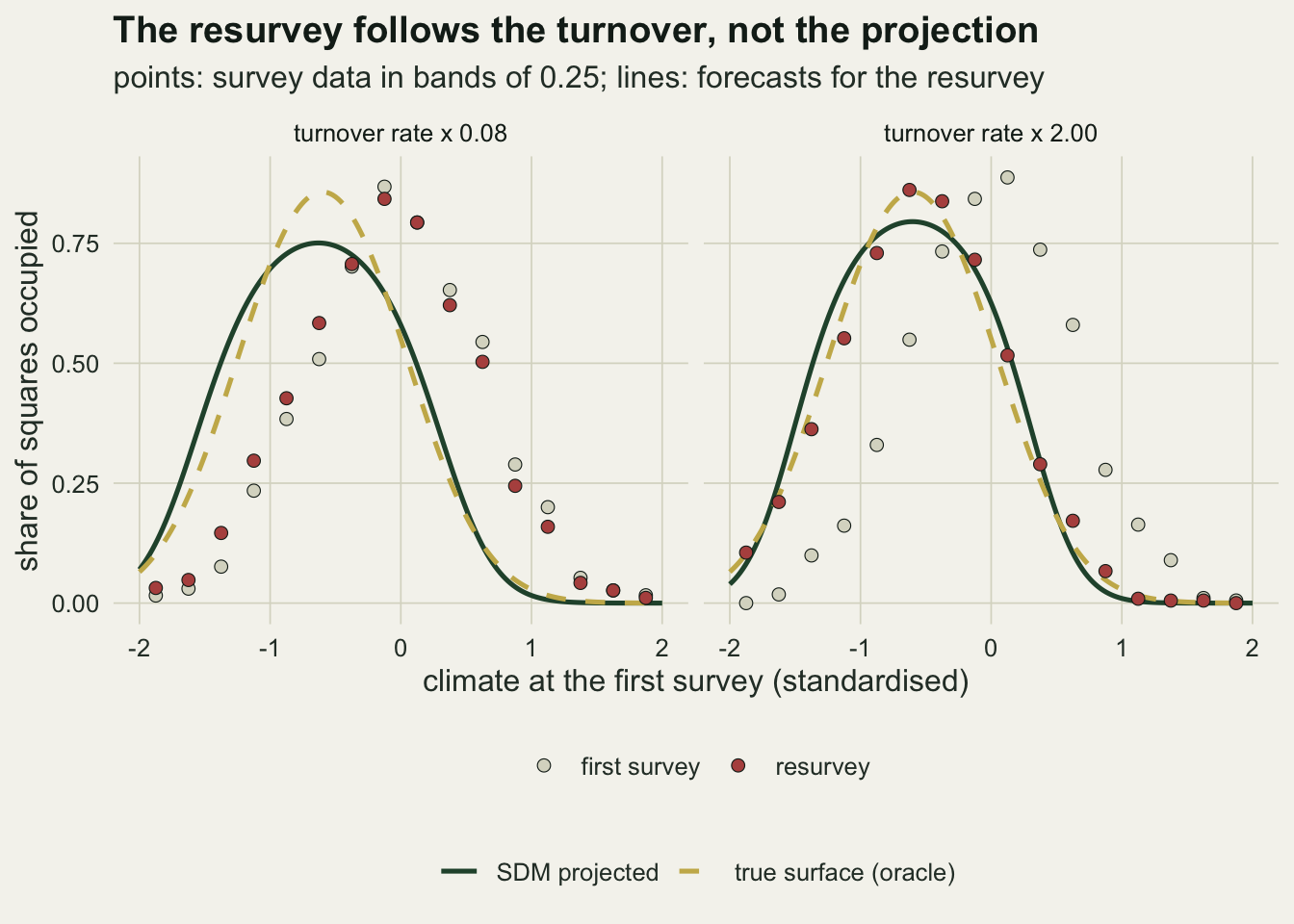

Figure 1: One landscape, two turnover rates: the share of squares occupied in each climate band at the first survey and at the resurvey, against the SDM fitted to the first survey and projected, and the true suitability surface at the warmed climate.

Scoring the resurvey across turnover rates

The sweep repeats the whole construction for each turnover rate: a fresh landscape, a first survey, a fitted SDM, a resurvey, and the four forecasts scored against it. The replication was fixed at two hundred landscapes per rate before anything ran, which puts the Monte Carlo standard error of every mean TSS near a thousandth.

n_rep <- 200
set.seed(9021)
runs_eq <- run_grid(lag = FALSE, n_rep = n_rep)

tab_eq <- data.frame(rate = rate_grid, turnover = grid_mean(runs_eq, "turnover"),
  sdm = grid_mean(runs_eq, "sdm_tss"), oracle = grid_mean(runs_eq, "oracle_tss"),
  persist = grid_mean(runs_eq, "persist_tss"), dynamic = grid_mean(runs_eq, "dynamic_tss"),
  sdm_b = grid_mean(runs_eq, "sdm_brier"), oracle_b = grid_mean(runs_eq, "oracle_brier"),
  persist_b = grid_mean(runs_eq, "persist_brier"), dynamic_b = grid_mean(runs_eq, "dynamic_brier"))
se_tss_max <- max(vapply(c("sdm_tss", "oracle_tss", "persist_tss", "dynamic_tss"),
                         function(k) max(grid_se(runs_eq, k)), 0))

gap_so_tss   <- tab_eq$sdm - tab_eq$oracle
gap_so_se    <- diff_se(runs_eq, "sdm_tss", "oracle_tss")
gap_so_z     <- max(abs(gap_so_tss) / gap_so_se)
gap_so_brier <- tab_eq$sdm_b - tab_eq$oracle_b
gap_sob_se   <- diff_se(runs_eq, "sdm_brier", "oracle_brier")
gap_sob_z    <- gap_so_brier / gap_sob_se

sp_gap   <- tab_eq$sdm - tab_eq$persist
sp_se    <- diff_se(runs_eq, "sdm_tss", "persist_tss")
cross_tss <- approx(sp_gap, tab_eq$turnover, xout = 0)$y
n_pers_win <- sum(sp_gap < 0)
stopifnot(all(sp_gap[seq_len(n_pers_win)] < 0))

brier_ident <- max(vapply(runs_eq, function(a) max(abs(a["persist_brier", ] - a["turnover", ])), 0))
stopifnot(brier_ident < 1e-12)
cross_brier <- approx(tab_eq$sdm_b - tab_eq$persist_b, tab_eq$turnover, xout = 0)$y

num_word  <- c("one", "two", "three", "four", "five", "six")
dyn_best  <- all(tab_eq$dynamic_b < pmin(tab_eq$sdm_b, tab_eq$oracle_b, tab_eq$persist_b))
dyn_gain_fast <- tab_eq$sdm_b[6] - tab_eq$dynamic_b[6]
dyn_gain_se   <- diff_se(runs_eq, "sdm_brier", "dynamic_brier")[6]
dyn_orc_fast  <- tab_eq$oracle_b[6] - tab_eq$dynamic_b[6]
dyn_is_pers   <- vapply(runs_eq, function(a) all(a["dynamic_tss", ] == a["persist_tss", ]), TRUE)
n_dyn_pers    <- sum(dyn_is_pers)
stopifnot(dyn_best, all(dyn_is_pers[seq_len(n_dyn_pers)]))
peek_gain <- grid_mean(runs_eq, "sdm_peek") - tab_eq$sdm
peek_min  <- min(vapply(runs_eq, function(a) min(a["sdm_peek", ] - a["sdm_tss", ]), 0))
stopifnot(peek_min >= 0, min(peek_gain) > max(abs(gap_so_tss)))

# the rank identity: SDM map = true surface re-centred on the fitted optimum
rc_check <- function(runs) c(
  curv  = max(vapply(runs, function(a) max(a["curv", ]), 0)),
  ndiff = max(vapply(runs, function(a) max(a["rc_ndiff", ]), 0)),
  tss   = max(vapply(runs, function(a) max(abs(a["sdm_tss", ] - a["rc_tss", ])), 0)))
rc_eq <- rc_check(runs_eq)
stopifnot(rc_eq["curv"] < 0, rc_eq["tss"] < 1e-3)
n_land   <- n_rep * length(rate_grid)
peak_rng <- range(grid_mean(runs_eq, "peak_sdm"))
opt_eq   <- grid_mean(runs_eq, "opt_fit")
opt_sd   <- max(vapply(runs_eq, function(a) sd(a["opt_fit", ]), 0))

On the binary maps the SDM and the oracle are the same forecast, and for a reason that needs no simulation. On one climate axis both are bell-shaped curves, symmetric about their optimum: the true surface falls with distance from zero, and the fitted quadratic logistic falls with distance from its own fitted optimum whenever its squared term is negative, which it is in every landscape here. Ranking the first-survey squares by either curve is therefore ranking them by distance from the optimum, and a cut-off chosen by maximum TSS on the first survey picks the band of squares nearest the optimum that best separates the first survey’s presences from its absences, whatever the height or width of the curve. Projected onto the warmed climate, the map marks every square whose new climate falls in the same band around the same optimum. So the SDM’s binary map is the one the true surface would give if it were re-centred on the SDM’s fitted optimum. The chunk builds that re-centred map in every one of the 1200 landscapes, and the largest number of squares in which it disagrees with the SDM’s map, in any landscape, is 0. (The two could disagree only on a resurvey square whose climate falls between the two first-survey squares on either side of the cut-off.) The SDM’s TSS and extirpation recall can therefore differ from the oracle’s only through the error in its fitted optimum. The mean fitted optimum over the two hundred landscapes sat within 0.002 of zero at every rate, with a standard deviation between single landscapes of at most 0.018, and an error that small costs little: the largest difference in mean TSS between the SDM and the oracle is 0.0016, and the largest of the six paired differences is 2.0 standard errors. That agreement is the identity at work, not a measurement of how well a fitted model learns a niche.

The SDM’s probabilities are a different matter. The quadratic logistic curve is not the shape of the true equilibrium surface: the fitted peak averages between 0.763 and 0.766 across the rates, against 0.857 for the true surface. The Brier score picks that up in a direction that changes with the rate: the SDM’s Brier score is lower than the oracle’s by up to 0.0040 at the slow end and higher by up to 0.0021 at the fast end. Pairing the two forecasts on the same landscapes removes most of the noise, so these differences are up to 40 standard errors of the paired difference, but they are small next to the Brier gaps between the SDM and persistence, which run from 0.0225 to 0.205. Whatever the resurvey says about the SDM’s binary map, it says about the true suitability surface too, as long as the fitted optimum is right; the section on a lagging species below is about a case where it is not.

Persistence is where the verdict turns. At the slowest rate the old map scores a TSS of 0.846 against 0.381 for the SDM; at the fastest the order is reversed, 0.617 for the SDM against 0.250 for persistence. The old map wins at the three slowest rates and loses at the others, and interpolating linearly between grid points puts the crossover where 22.3 per cent of squares change state between the surveys. Below that, a model that knows the niche exactly is a worse forecast of the second atlas than the first atlas is. The Monte Carlo standard error of each of these means is at most 0.0014.

The Brier score draws the line somewhere else, and for a reason that needs no simulation. Persistence forecasts a probability of exactly one or zero, so its squared error is one for every square that changed state and zero for the rest, and its Brier score is the turnover share itself; the chunk checks that identity to machine precision. The SDM beats persistence on Brier score as soon as the turnover share exceeds the SDM’s own Brier score, which by linear interpolation happens at 17.4 per cent turnover, earlier than on TSS. Two scores, two crossovers: the TSS crossover and the Brier crossover are different quantities, and a report that quotes one should say which.

long_eq <- rbind(
  data.frame(turnover = tab_eq$turnover, score = "TSS (higher is better)",
             value = c(tab_eq$sdm, tab_eq$oracle, tab_eq$persist, tab_eq$dynamic),
             forecast = rep(c("SDM", "oracle", "persistence", "dynamic"), each = 6)),
  data.frame(turnover = tab_eq$turnover, score = "Brier score (lower is better)",
             value = c(tab_eq$sdm_b, tab_eq$oracle_b, tab_eq$persist_b, tab_eq$dynamic_b),
             forecast = rep(c("SDM", "oracle", "persistence", "dynamic"), each = 6)))
long_eq$score    <- factor(long_eq$score, levels = unique(long_eq$score))
long_eq$forecast <- factor(long_eq$forecast, levels = c("SDM", "oracle", "persistence", "dynamic"))

ggplot(long_eq, aes(turnover, value, colour = forecast, linetype = forecast)) +
  geom_line(linewidth = 0.9) +
  geom_point(size = 2) +
  facet_wrap(~ score, scales = "free_y") +
  scale_colour_manual(values = c(te_forest, te_gold, te_rust, te_ink), name = NULL) +
  scale_linetype_manual(values = c("solid", "dashed", "solid", "dotted"), name = NULL) +
  labs(x = "share of squares that changed state between the surveys", y = NULL,
       title = "The old map wins until the map turns over",
       subtitle = "thresholds from the first survey only; the dynamic forecast needs the true rates") +
  theme_datasheet() +
  theme(legend.position = "bottom")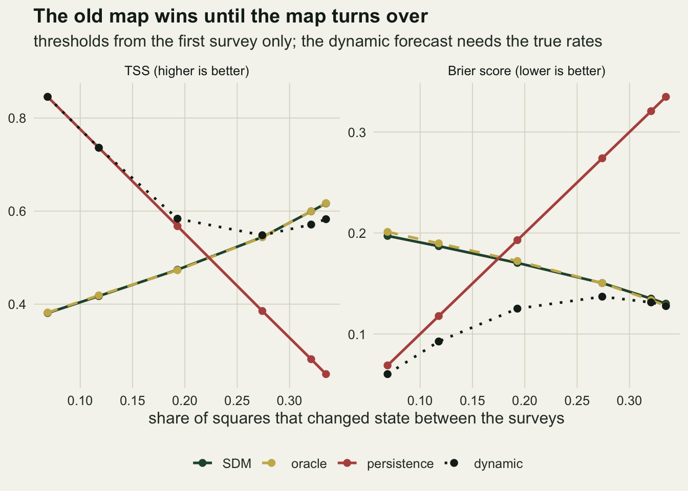

Figure 2: Mean TSS and Brier score of four forecasts of the resurvey against the share of squares that changed state, two hundred landscapes per turnover rate. Lower is better for the Brier score.

The dynamic forecast has the best Brier score at every rate; the chunk stops if that fails. At the slow end it is persistence with the edges softened, since a square that is occupied now is still occupied ten years later with a high probability, and at the two slowest rates its map at one half is the first survey exactly, in every landscape. At the fast end it has nearly forgotten the first survey and sits close to the equilibrium surface: its Brier score is 0.0003 below the oracle’s and 0.0024 below the SDM’s (standard error of the latter difference 0.0001). The middle of the range is where it earns its place, combining the current map with how fast that map decays. It is also the one forecast in the comparison that a single survey cannot produce: it needs colonisation and extinction rates, which is to say repeated surveys and a model like the one in dynamic occupancy: colonisation and extinction (MacKenzie et al. 2003), with detection handled, before the resurvey it is supposed to forecast.

One control on the thresholds. Had the SDM’s cut-off been tuned on the resurvey instead of the first survey, its mean TSS would have risen by 0.009 to 0.021 across the rates. The gain cannot be negative in any landscape, since the tuned cut-off is the best of all cut-offs on the same ranking, the one used above included; its size is the point. That is the flattery a threshold chosen with the answer in view adds, larger at every rate than any difference between the SDM and the oracle here, and it is the reason the thresholds above were fixed on the first survey.

Extirpation recall of a perfect niche map is well below one

The number most temporal validations report with regret is the share of observed extirpations that the projected map had written off. Here that share has a closed-form approximation: the expected number of losses in written-off squares over the expected number of losses, given the first survey. Given the first survey, a square occupied at the first survey loses the species by the second with a probability that follows from the chain, one minus the dynamic forecast for that square, and a fixed map writes off a given set of squares. The approximation is the probability-weighted share of losses that fall in written-off squares, sum(z0 * (1 - p) * (1 - b)) / sum(z0 * (1 - p)), with z0 the first survey, p the probability that a square is occupied at the resurvey given its state at the first, and b one where the map predicts presence. The chunk computes it for every landscape and compares it with the realised recall.

rec_tab <- data.frame(rate = rate_grid, turnover = tab_eq$turnover,
  sdm = grid_mean(runs_eq, "sdm_extrec"), oracle = grid_mean(runs_eq, "oracle_extrec"),
  oracle_exp = grid_mean(runs_eq, "oracle_extexp"), oracle_fx = grid_mean(runs_eq, "oracle_falsex"))
rec_se  <- grid_se(runs_eq, "oracle_extrec")
rec_gap <- max(abs(rec_tab$oracle - rec_tab$oracle_exp) / rec_se)
rec_so  <- max(abs(rec_tab$sdm - rec_tab$oracle))
rec_so_z <- max(abs(rec_tab$sdm - rec_tab$oracle) /
                  diff_se(runs_eq, "sdm_extrec", "oracle_extrec"))
miss_orc <- 1 - rec_tab$oracle
stopifnot(which.max(rec_tab$oracle_fx) == 1)
best_exp  <- grid_mean(runs_eq, "best_extexp")
best_gain <- best_exp - rec_tab$oracle_exp
stopifnot(all(best_gain >= 0))

The oracle catches between 0.551 and 0.582 of the extirpations across the rates, and the closed-form approximation agrees with the realised mean to within 1.2 Monte Carlo standard errors at every rate. The SDM’s recall differs from the oracle’s only through its fitted optimum, by the identity of the previous section, and the largest difference is 0.002, or 0.9 standard errors of the paired difference. So 42 to 45 per cent of the losses happen in squares that the true niche, projected perfectly, still calls suitable. They are the squares where extinction was a coin toss that came up the wrong way: the extinction probability is lowest at the optimum, but it is never zero.

Recall on its own has no ceiling: a map that writes off every square catches every loss. The ceiling that matters is recall at a fixed cost, and the same expression gives it. Among the squares occupied at the first survey, the map that writes off the ones with the highest true probability of loss scores highest on that expression of any map that writes off that many. Writing off as many occupied squares as the oracle does, it scores at most 0.013 above the oracle’s value of the same expression at any rate, in the mean over landscapes, so the oracle sits at or just below the best that any map can expect at its own write-off share, given the first survey.

The cost is not small. The same oracle map writes off 0.113 to 0.321 of the squares that kept the species, the most at the slowest rate, because a projected climate shift moves the whole predicted range and the trailing edge is predicted empty whether or not the populations there have gone yet. An SDM’s extirpation recall should be read against the oracle’s recall for the same threshold rule, and next to the share of persisting squares written off, never against one. The level of the ceiling in this construction is a property of the construction: another niche width, another shift or another extinction curve gives another number, and nothing here says what share of the shortfall in a real atlas is turnover and what share is the model.

rec_long <- rbind(
  data.frame(turnover = rec_tab$turnover, value = rec_tab$sdm,
             series = "SDM: losses caught"),
  data.frame(turnover = rec_tab$turnover, value = rec_tab$oracle,
             series = "oracle: losses caught"),
  data.frame(turnover = rec_tab$turnover, value = rec_tab$oracle_exp,
             series = "oracle: closed-form approximation"),
  data.frame(turnover = rec_tab$turnover, value = rec_tab$oracle_fx,
             series = "oracle: persisting squares written off"))
rec_long$series <- factor(rec_long$series, levels = unique(rec_long$series))

ggplot(rec_long, aes(turnover, value, colour = series, shape = series)) +
  geom_hline(yintercept = 1, colour = te_body, linetype = "dashed", linewidth = 0.5) +
  geom_line(linewidth = 0.8) +
  geom_point(size = 2.4) +
  scale_colour_manual(values = c(te_forest, te_gold, te_ink, te_rust), name = NULL) +
  scale_shape_manual(values = c(16, 17, 4, 15), name = NULL) +
  scale_y_continuous(limits = c(0, 1)) +
  labs(x = "share of squares that changed state between the surveys",
       y = "share",
       title = "A perfect niche model misses many losses",
       subtitle = "dashed line: a recall of one, reached only by writing off every square") +
  theme_datasheet() +
  theme(legend.position = "bottom") +
  guides(colour = guide_legend(nrow = 2), shape = guide_legend(nrow = 2))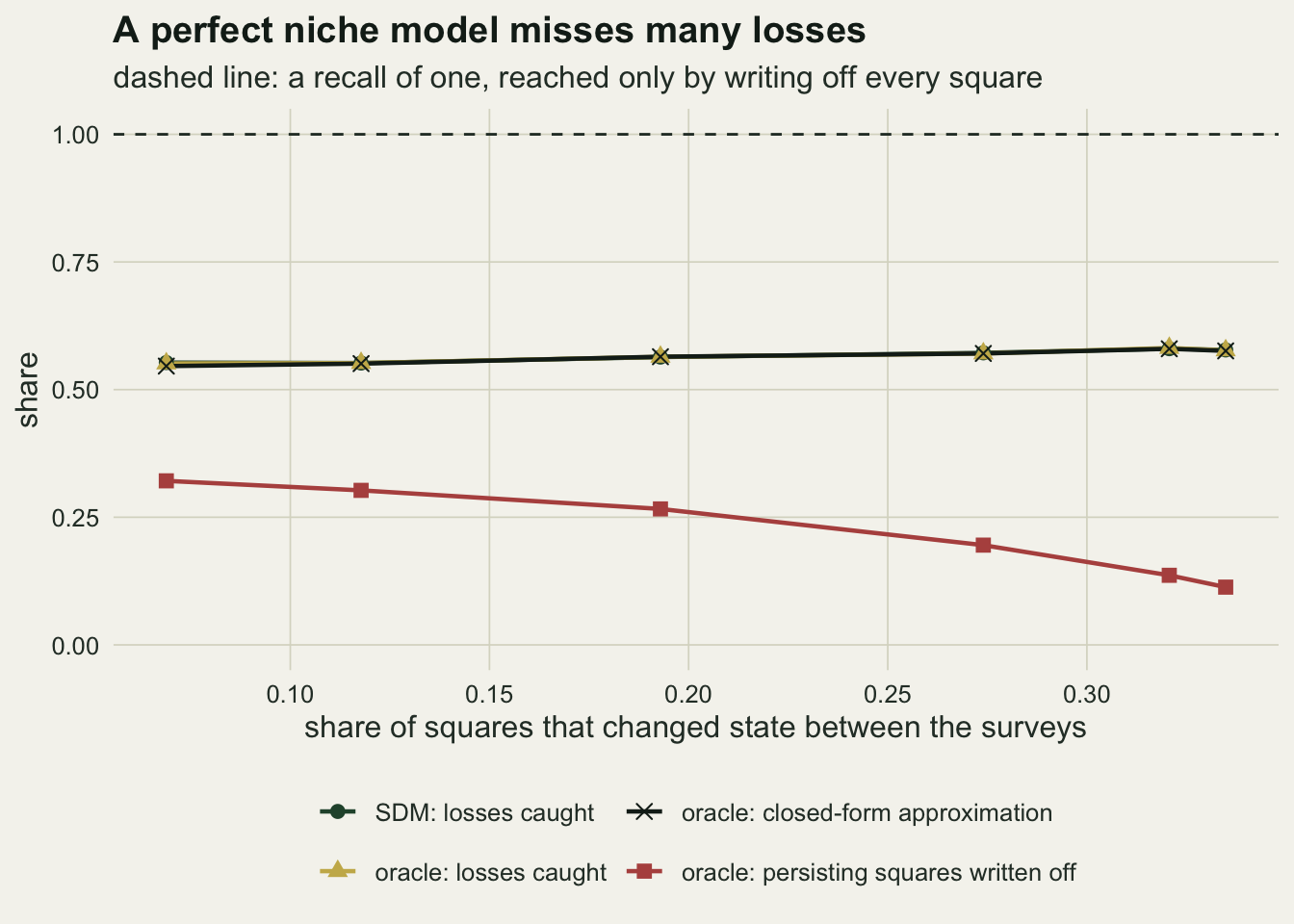

Figure 3: Extirpation recall of the projected SDM and of the true surface against the closed-form approximation, and the share of persisting squares the true surface wrote off, by turnover share.

A species that was already lagging

Everything above rests on one assumption the resurvey cannot check: that the species was at equilibrium with its climate when the first survey was taken. Elith, Kearney and Phillips (2010) discuss what that assumption costs when the modelled species is shifting its range, and a species with slow turnover in a warming climate is the obvious case, carrying what Kuussaari and colleagues (2009) call an extinction debt: populations still present in places that can no longer hold them in the long run. The second construction gives the species that history. It sat at the equilibrium of a climate 0.6 units cooler, warming began ten years before the first survey at the same speed as afterwards, and the first survey records wherever the species had got to. The SDM is fitted to that survey exactly as before. SDM fitted before the invasion is over measures the same failure at a leading edge, where a species still spreading has its fitted optimum on the climate of the founding site; the case here is a trailing edge, and the new question is what a resurvey then rewards. The identity above says where to look first: whether the fitted optimum still sits on the true one.

set.seed(6630)
runs_lag <- run_grid(lag = TRUE, n_rep = n_rep)
tab_lag <- data.frame(rate = rate_grid, turnover = grid_mean(runs_lag, "turnover"),
  sdm = grid_mean(runs_lag, "sdm_tss"), oracle = grid_mean(runs_lag, "oracle_tss"),
  persist = grid_mean(runs_lag, "persist_tss"), sdm_rec = grid_mean(runs_lag, "sdm_extrec"),
  oracle_rec = grid_mean(runs_lag, "oracle_extrec"), oracle_fx = grid_mean(runs_lag, "oracle_falsex"),
  opt_fit = grid_mean(runs_lag, "opt_fit"))
lag_so    <- tab_lag$sdm - tab_lag$oracle
lag_so_se <- diff_se(runs_lag, "sdm_tss", "oracle_tss")
lag_sp    <- tab_lag$sdm - tab_lag$persist
cross_lag <- approx(lag_sp, tab_lag$turnover, xout = 0)$y
n_lag_pers <- sum(lag_sp < 0)
stopifnot(all(lag_sp[seq_len(n_lag_pers)] < 0), which.max(tab_lag$opt_fit) == 1)
rc_lag <- rc_check(runs_lag)
stopifnot(rc_lag["curv"] < 0, rc_lag["tss"] < 1e-3)

It does not, and the direction is the uncomfortable one. At equilibrium the mean fitted optimum sat within 0.002 of the true optimum at zero at every rate. For the lagging species the mean over the two hundred landscapes sits at 0.513 at the slowest rate, 86 per cent of the way to the old optimum at 0.6, and at 0.033 at the fastest, where the species had nearly caught up. The SDM has fitted the lag as if it were the niche. The identity still holds: the largest number of squares in which the SDM’s map disagrees with the map of the true surface re-centred on its fitted optimum, in any lagging landscape, is 0, so everything below that separates the SDM from the oracle is the displacement of that optimum.

On the resurvey that mistake pays. At the slowest rate the SDM scores a TSS of 0.374 and the true suitability surface 0.041, a gap of 0.333 with a standard error of 0.0017. The oracle predicts the species where the climate says it should be, and ten years of slow turnover have not put it there; the SDM predicts it near where it was, and that is where it still is. The gap closes as the rate rises, and at the fastest rate its absolute value is 0.0001 with a standard error of 0.0005. The oracle’s extirpation recall at the slowest rate is 0.737 against 0.494 for the SDM, because it writes off the stranded trailing edge; it also writes off 0.522 of the squares that kept the species, which is why its TSS collapses.

Persistence still wins at the slow end, at the two slowest rates, with the TSS crossover at 23.4 per cent turnover. The figure puts the rate multiplier on its horizontal axis rather than the turnover share, because for this species the share is 0.3459 at a multiplier of 1.2 and 0.3428 at 2, which does not order the fast end. So the lagging case keeps the persistence result and breaks the equality, because the optimum has moved. A resurvey cannot tell a model of the niche from a model of the species’ recent history: with slow turnover it rewards the model that learned the lag and punishes the one that knows the niche, and a good resurvey score then shows that the model reproduces where the species still is, not that the niche was estimated correctly.

long_lag <- data.frame(rate = rate_grid,
                       value = c(tab_lag$sdm, tab_lag$oracle, tab_lag$persist),
                       forecast = rep(c("SDM", "oracle", "persistence"), each = 6))
long_lag$forecast <- factor(long_lag$forecast, levels = c("SDM", "oracle", "persistence"))
opt_lab <- data.frame(rate = rate_grid, value = tab_lag$sdm,
                      label = sprintf("%.2f", tab_lag$opt_fit))

ggplot(long_lag, aes(rate, value, colour = forecast, linetype = forecast)) +
  geom_line(linewidth = 0.9) +
  geom_point(size = 2) +
  geom_text(data = opt_lab, aes(rate, value, label = label), inherit.aes = FALSE,
            colour = te_forest, size = 3.4, vjust = -1.1) +
  scale_colour_manual(values = c(te_forest, te_gold, te_rust), name = NULL) +
  scale_linetype_manual(values = c("solid", "dashed", "solid"), name = NULL) +
  scale_x_log10(breaks = rate_grid) +
  scale_y_continuous(limits = c(0, 1)) +
  labs(x = "turnover rate multiplier (log scale)", y = "TSS on the resurvey",
       title = "A lagging species: the fitted model beats the true niche",
       subtitle = "labels: the SDM's mean fitted optimum; the true optimum is zero") +
  theme_datasheet() +
  theme(legend.position = "bottom")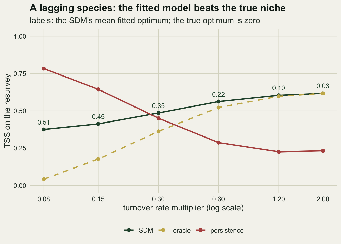

Figure 4: The lagging species: mean TSS of the SDM, the true suitability surface and persistence on the resurvey, against the turnover rate multiplier on a log scale, two hundred landscapes per rate; the SDM’s mean fitted optimum is printed above each SDM point.

A longer interval

The crossover above was measured for a resurvey ten years after the first survey, with all the warming inside that interval. The interval is a design choice of the construction, so it was changed once: the same equilibrium sweep with the resurvey after twenty years, the climate holding still for the second decade.

set.seed(7702)
runs_20 <- run_grid(lag = FALSE, n_rep = 100, t_res = 20)
turn_20 <- grid_mean(runs_20, "turnover")
sp_20   <- grid_mean(runs_20, "sdm_tss") - grid_mean(runs_20, "persist_tss")
cross_20_turn <- approx(sp_20, turn_20, xout = 0)$y
cross_10_rate <- exp(approx(sp_gap, log(rate_grid), xout = 0)$y)
cross_20_rate <- exp(approx(sp_20, log(rate_grid), xout = 0)$y)
so_20 <- max(abs(grid_mean(runs_20, "sdm_tss") - grid_mean(runs_20, "oracle_tss")))
n_pers_20 <- sum(sp_20 < 0)
stopifnot(all(sp_20[seq_len(n_pers_20)] < 0), all(sp_20[-seq_len(n_pers_20)] > 0),
          all(sp_gap[-seq_len(n_pers_win)] > 0))
brk_10 <- 100 * tab_eq$turnover[n_pers_win + 0:1]
brk_20 <- 100 * turn_20[n_pers_20 + 0:1]

With twenty years between the surveys the crossover moves to a slower species: on the rate multiplier, interpolated on a log scale, it falls from 0.39 to 0.17. In units of turnover share it barely moves: 22 per cent at twenty years and 22 per cent at ten. Both are linear interpolations between the grid points that bracket them, 20.5 and 28.8 per cent turnover at twenty years and 19.3 and 27.4 at ten, so the two shares agree to within the spacing of the grid and no more finely than that. The share of squares that changed state between the two surveys is the better guide to which forecast wins, and the rate per year is not; the climate path also differs between the two intervals, so this is a reading of one construction rather than a law. The SDM and the oracle still differ by at most 0.002 in mean TSS, as the identity says they must while the fitted optimum is right.

What to report

Report the resurvey score of the old map beside the score of the model. Persistence costs nothing to compute and it is the hard baseline whenever squares change hands slowly; a model that loses to it has not shown that it forecasts change, whatever its TSS on the first survey was. Report the share of squares that changed state between the surveys as well, since it tells a reader which side of the crossover the comparison sits on.

Choose every threshold on the first survey, say that you did, and say what the rule was. A cut-off tuned on the resurvey flatters the model, here by more than any difference between the SDM and the true niche in the equilibrium sweep.

Report extirpation recall together with the share of persisting squares the map wrote off, and read both against what a perfect suitability map would have scored. Under stochastic turnover the best recall any map can expect at a given number of occupied squares written off is below one; it can be computed from any fitted dynamic model with the expression above, and a recall well below one can be that ceiling rather than the model. Say which score a verdict rests on: the TSS and the Brier score crossed at different turnover shares here.

State whether the species can be assumed to be at equilibrium at the first survey, and why. If it was lagging, a good resurvey score is not evidence that the niche was estimated well, and a fitted optimum displaced towards the climate the species used to occupy is the thing to look for, the trailing-edge version of the founding-climate check that SDM fitted before the invasion is over runs, and finds one-sided, at a leading edge. If repeated surveys exist before the resurvey, fit colonisation and extinction and use the dynamic forecast; it was the best forecast on the Brier score at every rate here.

Honest limits

Detection is perfect. Every square is visited in both surveys and every occupied square is recorded, so every change between the atlases is a real change. Real resurveys mix real losses with missed detections, and missed detections look like extirpations to every score here; checking a range shift analysis and the occupancy posts are where that problem is measured.

There is one climate variable and the SDM has the matching quadratic. Its probabilities are not the true ones (its peak is too low), but its thresholded maps depend only on where its optimum sits, which is why it matches the oracle on TSS and recall; that match is an identity of this construction, not evidence that fitted models recover niches. With several covariates, an asymmetric response or a cut-off fixed on the probability scale instead of chosen by ranking, the identity breaks, and a real model with the wrong covariates, or a flexible one that overfits the first survey, can sit below the oracle, and then a low resurvey score is partly the model. The point here is only that the oracle’s score, not one, is the target.

Squares are independent. Colonisation does not depend on occupied neighbours, so there is no dispersal limit and no front. A species that must spread into newly suitable squares from occupied ones would colonise them more slowly than this one, which should widen the slow-turnover regime where persistence wins and adds a spatial lag the SDM cannot see; that case was not run.

The dynamic forecast uses the true rates and the true climate path. A fitted dynamic model has estimation error in both rates and needs a forecast of the climate, so its advantage here is an upper bound. Its binary map at one half is not the TSS-optimal cut-off for it, which is why its TSS falls below the SDM’s at the fast end while its Brier score stays the lowest; the Brier score is the fair comparison for it.

The lagging species has one history: warming for ten years before the first survey at the same speed as afterwards. A longer or faster history should strand more of the range and widen the gap between the SDM and the oracle, and a shorter one narrow it; only the one history was run. The crossover location and the ceiling on recall are properties of this niche, this shift and this extinction curve. The direction of each result is what carries over, not its size.

References

Rapacciuolo G, Roy DB, Gillings S, Fox R, Walker K, Purvis A 2012 PLoS ONE 7(7):e40212 (10.1371/journal.pone.0040212)

Auffret AG, Nenzen HK, Polaina E 2024 Diversity and Distributions 30(7):e13834 (10.1111/ddi.13834)

Allouche O, Tsoar A, Kadmon R 2006 Journal of Applied Ecology 43(6):1223-1232 (10.1111/j.1365-2664.2006.01214.x)

Elith J, Kearney M, Phillips S 2010 Methods in Ecology and Evolution 1(4):330-342 (10.1111/j.2041-210X.2010.00036.x)

Kuussaari M, Bommarco R, Heikkinen RK, et al. 2009 Trends in Ecology and Evolution 24(10):564-571 (10.1016/j.tree.2009.04.011)

MacKenzie DI, Nichols JD, Hines JE, Knutson MG, Franklin AB 2003 Ecology 84(8):2200-2207 (10.1890/02-3090)

Related tutorials

• Forecast skill and the baseline
• Evaluating species distribution models in R
• Occupancy turnover and equilibrium
• SDM fitted before the invasion is over