---
title: "Dynamic occupancy: colonisation and extinction"
description: "Fit a multi-season occupancy model in base R with a forward likelihood, and see why naive year-to-year turnover confounds extinction with imperfect detection."
date: "2026-05-22 10:00"
categories: [occupancy, ecology tutorial, R, population dynamics]
image: thumbnail.png
image-alt: "Occupancy declining across six seasons toward an equilibrium line, with the modelled curve tracking the truth and naive observed occupancy sitting below it."
---
A single-season occupancy model (see [single-season occupancy](../single-season-occupancy-model/)) gives one snapshot: the probability a site is occupied, corrected for the fact that you miss the species sometimes. Most monitoring runs longer than one season, and the interesting question is not the snapshot but the change. Did a patch lose the species? Was an empty patch colonised? Comparing the raw detections year to year answers that badly, because a site where you simply failed to detect an occupied species looks exactly like a local extinction.
The dynamic (multi-season) occupancy model of MacKenzie et al. (2003) separates the two. Sites are surveyed in several primary periods (seasons), and within each season a handful of repeat visits carry the detection information. Between seasons the occupancy state follows a two-state Markov chain: an occupied site persists or goes locally extinct, an empty site stays empty or is colonised. The whole thing is a hidden Markov model, and the likelihood is the same scaled forward pass used for [multi-state capture-recapture](../multistate-capture-recapture/), only here the two states are "occupied" and "empty" and the seasons play the role of occasions.
## The model
Four parameters describe a homogeneous system. Initial occupancy `psi1` sets the state in season one. Colonisation `gamma` is the probability an empty site becomes occupied by the next season; local extinction `eps` is the probability an occupied site becomes empty. Detection `p` is the per-visit probability of recording the species given the site is occupied. The state transition matrix, with rows the state now and columns the state next season, is
```
        empty     occupied
empty   1 - gamma   gamma
occ.    eps         1 - eps
```
Within a season the repeat visits are independent Bernoulli detections: an occupied site produces a detection with probability `p` on each of the `K` visits, an empty site never produces one. The equilibrium occupancy this Markov chain drifts toward is `gamma / (gamma + eps)`, and if you start away from it you get a trend even though the rates never change.
## Simulate a data set
Two hundred and fifty sites, six seasons, four visits each. Colonisation is slower than extinction, so occupancy starts above equilibrium and declines toward it.
```{r}
#| label: sim
set.seed(139)
R <- 250; Tn <- 6; K <- 4
psi1 <- 0.55; gamma <- 0.20; eps <- 0.30; p <- 0.35

z <- matrix(0L, R, Tn)               # latent occupancy state
z[, 1] <- rbinom(R, 1, psi1)
for (t in 2:Tn) z[, t] <- rbinom(R, 1, ifelse(z[, t - 1] == 1, 1 - eps, gamma))

d <- matrix(0L, R, Tn)               # detections per season (out of K)
for (t in 1:Tn) d[, t] <- rbinom(R, K, z[, t] * p)

round(gamma / (gamma + eps), 3)      # equilibrium occupancy
```
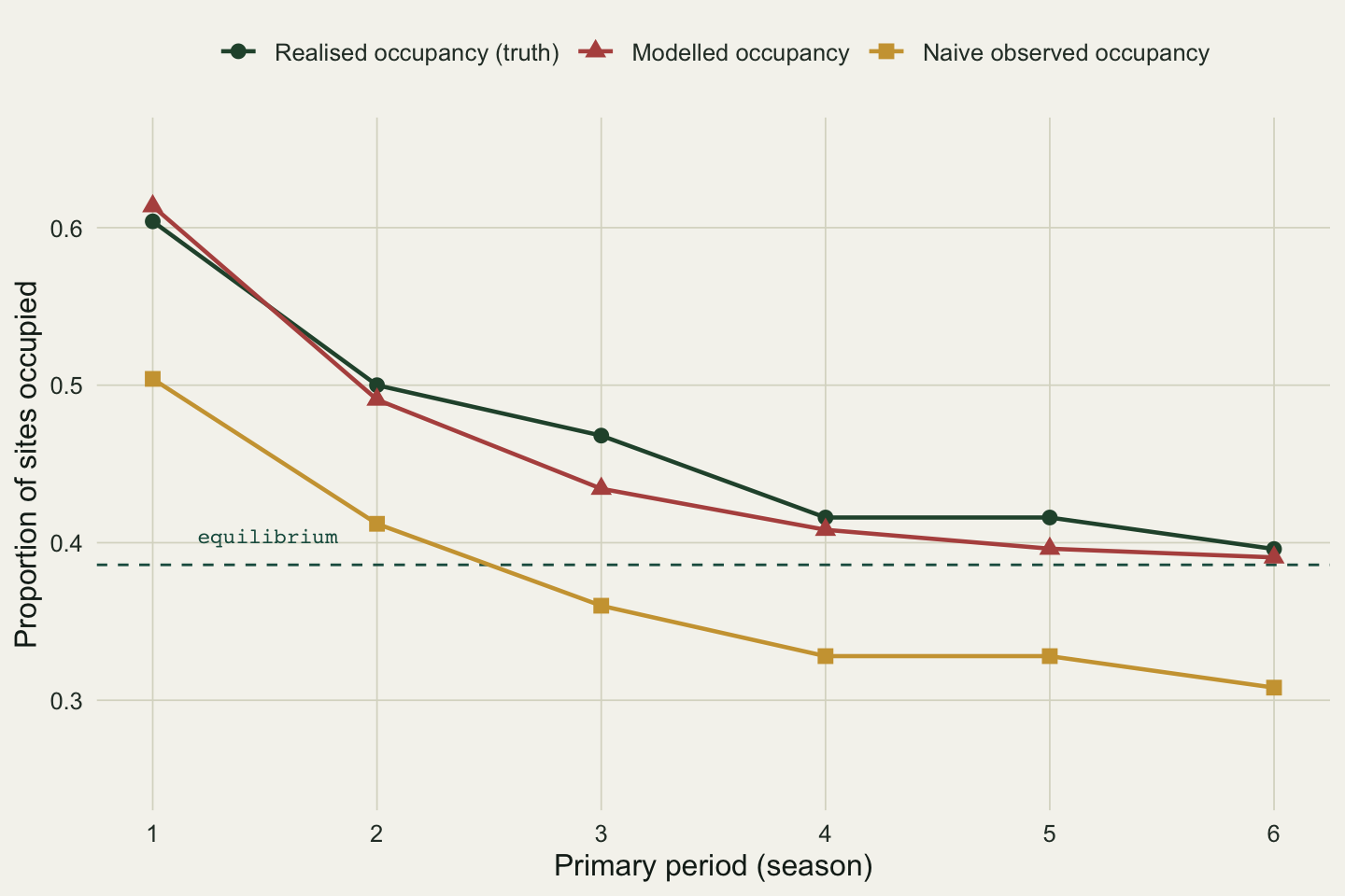
The equilibrium the chain heads for is 0.400. The realised occupancy (the fraction of sites truly occupied, which you never see in the field) falls from 0.604 in season one to 0.396 in season six.
## The forward likelihood by hand
For one site, the forward algorithm carries a length-two vector of state probabilities across seasons, multiplying by the emission at each season and by the transition matrix between seasons. Scaling at every step keeps the numbers away from underflow and hands you the log-likelihood as the sum of the log scaling constants. The emission for an occupied site is `p^d (1 - p)^(K - d)`; for an empty site it is one if there were no detections and zero otherwise.
```{r}
#| label: likelihood
emit <- function(dt, p, K) c(as.numeric(dt == 0), p^dt * (1 - p)^(K - dt))

site_ll <- function(dv, init, Phi, p, K) {
  a <- init * emit(dv[1], p, K); s <- sum(a); ll <- log(s); a <- a / s
  for (t in 2:length(dv)) {
    a <- as.vector(a %*% Phi) * emit(dv[t], p, K)
    s <- sum(a); ll <- ll + log(s); a <- a / s
  }
  ll
}

nll <- function(par) {
  ps <- plogis(par[1]); ga <- plogis(par[2]); ep <- plogis(par[3]); pp <- plogis(par[4])
  Phi <- matrix(c(1 - ga, ga, ep, 1 - ep), 2, 2, byrow = TRUE)
  -sum(apply(d, 1, site_ll, init = c(1 - ps, ps), Phi = Phi, p = pp, K = K))
}

fit <- optim(c(0, qlogis(0.2), qlogis(0.2), qlogis(0.3)), nll,
             method = "BFGS", hessian = TRUE)
stopifnot(fit$convergence == 0)   # check before inverting the Hessian
est <- plogis(fit$par); names(est) <- c("psi1", "gamma", "eps", "p")
se  <- sqrt(diag(solve(fit$hessian))) * est * (1 - est)   # delta-method SE
round(rbind(estimate = est, se = se), 3)
```
Optimising the four parameters on the logit scale and back-transforming, the estimates are `psi1` 0.614 (SE 0.038), `gamma` 0.208 (SE 0.020), `eps` 0.331 (SE 0.028) and `p` 0.347 (SE 0.012). All four true values sit inside the Wald intervals in this fit; colonisation and detection are recovered almost exactly and extinction to within about one standard error, and the initial occupancy estimate matches the realised season-one fraction of 0.60. With `p` at 0.35 and four visits, an occupied site is detected at least once with probability `1 - (1 - 0.347)^4 = 0.818`, so roughly one occupied site in five slips through undetected in any given season.
## What the naive comparison gets wrong
The tempting shortcut is to treat a detection as occupancy and read turnover straight off the observed histories: count how often a site that looked empty last season looks occupied this season (apparent colonisation) and how often an occupied-looking site goes quiet (apparent extinction).
```{r}
#| label: naive-turnover
obs <- (d > 0) * 1L
cn <- cd <- en <- ed <- 0
for (t in 2:Tn) {
  u0 <- obs[, t - 1] == 0; o1 <- obs[, t - 1] == 1
  cd <- cd + sum(u0); cn <- cn + sum(u0 & obs[, t] == 1)
  ed <- ed + sum(o1); en <- en + sum(o1 & obs[, t] == 0)
}
c(naive_colonisation = round(cn / cd, 3), naive_extinction = round(en / ed, 3))
```
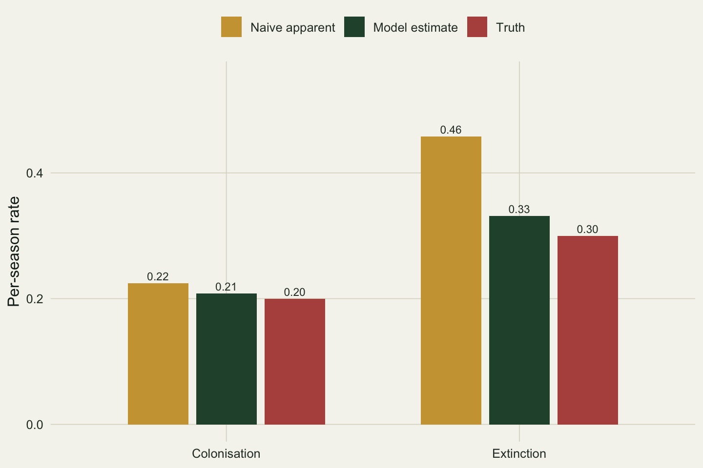
Apparent colonisation comes out at 0.224 against a truth of 0.20, a mild overstatement. Apparent extinction is 0.458 against a truth of 0.30, a much larger one. The asymmetry is the whole point. An occupied site that you fail to detect this season is scored as an extinction, and there are many occupied sites to miss, so the extinction rate inflates. Empty sites cannot be detected by accident, so colonisation is biased far less. The model's own estimates, 0.208 and 0.331, land close to the truth because the likelihood already accounts for the visits where an occupied site went unseen.
```{r}
#| label: fig-trajectory
#| fig-cap: "Occupancy across six seasons: the true (realised) proportion occupied, the model-implied trajectory from the fitted rates, and the naive observed proportion. The dashed line marks the estimated equilibrium."
#| fig-alt: "Line plot of occupancy against season. Realised and modelled occupancy fall from about 0.60 to 0.39 and level off near the dashed equilibrium at 0.39. Naive observed occupancy has the same shape but sits about 0.08 to 0.10 lower throughout."
#| fig-width: 7.5
#| fig-height: 5.0
suppressMessages({library(ggplot2); library(dplyr)})
theme_te <- function(bs = 12) theme_minimal(base_size = bs) + theme(
  plot.background = element_rect(fill = "#f5f4ee", colour = NA),
  panel.background = element_rect(fill = "#f5f4ee", colour = NA),
  panel.grid.major = element_line(colour = "#dad9ca", linewidth = 0.3),
  panel.grid.minor = element_blank(),
  axis.text = element_text(colour = "#2c3a31"), axis.title = element_text(colour = "#16241d"),
  plot.title = element_text(colour = "#16241d", face = "bold"),
  plot.subtitle = element_text(colour = "#46604a"),
  legend.text = element_text(colour = "#2c3a31"), legend.position = "top",
  legend.key = element_rect(fill = "#f5f4ee", colour = NA))

psit <- numeric(Tn); psit[1] <- est["psi1"]
for (t in 2:Tn) psit[t] <- psit[t - 1] * (1 - est["eps"]) + (1 - psit[t - 1]) * est["gamma"]
psi_eq <- unname(est["gamma"] / (est["gamma"] + est["eps"]))

traj <- bind_rows(
  data.frame(season = 1:Tn, occ = colMeans(z),     series = "Realised occupancy (truth)"),
  data.frame(season = 1:Tn, occ = psit,            series = "Modelled occupancy"),
  data.frame(season = 1:Tn, occ = colMeans(d > 0), series = "Naive observed occupancy"))
traj$series <- factor(traj$series,
  levels = c("Realised occupancy (truth)", "Modelled occupancy", "Naive observed occupancy"))

ggplot(traj, aes(season, occ, colour = series, shape = series)) +
  geom_hline(yintercept = psi_eq, linetype = "dashed", colour = "#1d5b4e", linewidth = 0.5) +
  annotate("text", x = 1.2, y = psi_eq + 0.018, label = "equilibrium",
           colour = "#1d5b4e", size = 3, hjust = 0, family = "mono") +
  geom_line(linewidth = 0.8) + geom_point(size = 2.6) +
  scale_colour_manual(values = c("Realised occupancy (truth)" = "#275139",
    "Modelled occupancy" = "#b5534e", "Naive observed occupancy" = "#cda23f")) +
  scale_shape_manual(values = c("Realised occupancy (truth)" = 16,
    "Modelled occupancy" = 17, "Naive observed occupancy" = 15)) +
  scale_x_continuous(breaks = 1:Tn) + coord_cartesian(ylim = c(0.25, 0.65)) +
  labs(x = "Primary period (season)", y = "Proportion of sites occupied",
       colour = NULL, shape = NULL) +
  theme_te() + guides(colour = guide_legend(nrow = 1))
```
The modelled trajectory (from the recursion `psi[t] = psi[t-1] (1 - eps) + (1 - psi[t-1]) gamma`) sits right on the realised one and settles at the estimated equilibrium of 0.386. The naive series keeps the shape but rides about 0.08 to 0.10 below throughout: a constant deflation that a reader could easily mistake for a stronger decline if they had nothing to compare it against.
```{r}
#| label: fig-turnover
#| fig-cap: "Per-season colonisation and extinction from the naive apparent counts, the fitted model, and the truth. Extinction is the rate that the naive approach inflates."
#| fig-alt: "Grouped bar chart of colonisation and extinction rates for three sources. For colonisation the three bars are close (0.22, 0.21, 0.20). For extinction the naive bar is 0.46 while the model and truth bars are 0.33 and 0.30."
#| fig-width: 7.5
#| fig-height: 5.0
tr <- data.frame(
  rate = rep(c("Colonisation", "Extinction"), 3),
  source = rep(c("Naive apparent", "Model estimate", "Truth"), each = 2),
  value = c(cn / cd, en / ed, est["gamma"], est["eps"], gamma, eps))
tr$source <- factor(tr$source, levels = c("Naive apparent", "Model estimate", "Truth"))

ggplot(tr, aes(rate, value, fill = source)) +
  geom_col(position = position_dodge(0.7), width = 0.62) +
  scale_fill_manual(values = c("Naive apparent" = "#cda23f",
    "Model estimate" = "#275139", "Truth" = "#b5534e")) +
  geom_text(aes(label = sprintf("%.2f", value)), position = position_dodge(0.7),
            vjust = -0.4, size = 3, colour = "#2c3a31") +
  coord_cartesian(ylim = c(0, 0.55)) +
  labs(x = NULL, y = "Per-season rate", fill = NULL) +
  theme_te()
```
## Where this leaves you
A multi-season occupancy model buys three things a stack of single-season fits cannot. It gives colonisation and extinction as parameters rather than as artefacts of missed visits, it produces an equilibrium and a trajectory you can project, and it does both from the same repeat-visit data you already collect. The rates here are constant across sites and seasons, which is rarely the case in a real study: the next step is to let colonisation, extinction and detection depend on covariates, which is where [dynamic occupancy with covariates](../dynamic-occupancy-covariates/) picks up. From the fitted rates you can read the [occupancy trajectory and turnover](../occupancy-turnover-and-equilibrium/), and before trusting any of it you should ask whether the constant-detection assumption holds, which is the job of [checking a dynamic occupancy model](../checking-a-dynamic-occupancy-model/).
## References
- MacKenzie, Nichols, Hines, Knutson, Franklin 2003. Ecology 84(8):2200-2207 (10.1890/02-3090).
- MacKenzie, Nichols, Lachman, Droege, Royle, Langtimm 2002. Ecology 83(8):2248-2255 (10.1890/0012-9658(2002)083[2248:ESORWD]2.0.CO;2).
- Royle, Kery 2007. Ecology 88(7):1813-1823 (10.1890/06-0669.1).
- MacKenzie, Nichols, Royle, Pollock, Bailey, Hines 2018. Occupancy Estimation and Modeling, 2nd ed. ISBN 978-0-12-407197-1.
## Related tutorials
- [Single-season occupancy model](../single-season-occupancy-model/)
- [Neighbourhood colonisation and false jumps](../neighbourhood-colonisation-and-false-jumps/)
- [Occupancy turnover and equilibrium](../occupancy-turnover-and-equilibrium/)
- [Checking a dynamic occupancy model](../checking-a-dynamic-occupancy-model/)