---
title: "Checking a dynamic occupancy model"
description: "Test the fit of a dynamic occupancy model in base R with a parametric bootstrap, and catch the detection heterogeneity that leaves the estimates looking fine."
date: "2026-05-22 13:00"
categories: [occupancy, ecology tutorial, R, population dynamics]
image: thumbnail.png
image-alt: "Two histograms of a bootstrap chi-square statistic. In the first the observed value sits inside the cloud; in the second it lies to the right of every bootstrap value."
date-modified: "2026-09-27"
---
*Corrected 27 September 2026: the preview image came from an older run whose c-hat values and observed statistic did not match the post; it is now drawn from the post's own bootstrap figure.*
The three preceding tutorials fit dynamic occupancy models and read quantities out of them, all on the assumption that the model is right. A converged fit with tight standard errors says nothing about whether the model describes the data: it can be confidently wrong. The recurring worry for occupancy models is among-site variation in detection that the model does not include, some sites simply being easier to survey than others. That heterogeneity can leave colonisation and extinction looking reasonable while quietly biasing them, and the only way to find it is to test the fit directly. The tool is the parametric-bootstrap goodness-of-fit check of MacKenzie and Bailey (2004), and it closes this series the way [checking multi-state models](../checking-multistate-models/) closed the capture-recapture one.
## Two data sets, one model
Build two data sets over the same design of four hundred sites, five seasons and four visits. The first has a single detection probability for every site. The second splits the sites into two groups, one easy to detect and one hard, with the same average detection. Both are fitted with the same constant-detection model.
```{r}
#| label: setup
Tn <- 5; K <- 4; R <- 400; psi1 <- 0.55; gamma <- 0.20; eps <- 0.25; M <- Tn * K
Hgrid <- as.matrix(expand.grid(rep(list(0:K), Tn)))   # every possible count history
tot_grid <- rowSums(Hgrid)

fwd_ll <- function(H, pr, K) {                         # log P(count history), vectorised over rows
  ps <- pr[1]; ga <- pr[2]; ep <- pr[3]; pp <- pr[4]
  Phi <- matrix(c(1 - ga, ga, ep, 1 - ep), 2, 2, byrow = TRUE); n <- nrow(H)
  em <- function(t) { dc <- H[, t]; cbind(as.numeric(dc == 0), dbinom(dc, K, pp)) }
  a <- matrix(c(1 - ps, ps), n, 2, byrow = TRUE) * em(1); s <- rowSums(a); ll <- log(s); a <- a / s
  for (t in 2:ncol(H)) { a <- (a %*% Phi) * em(t); s <- rowSums(a); ll <- ll + log(s); a <- a / s }
  ll
}
nll    <- function(par, d, K) -sum(fwd_ll(d, plogis(par), K))
fitfun <- function(d) optim(c(0, qlogis(0.2), qlogis(0.2), qlogis(0.3)), nll,
                            d = d, K = K, method = "BFGS")
gen <- function(pvec, ps = psi1, ga = gamma, ep = eps) {   # dynamics default to the truth
  z <- matrix(0L, R, Tn); z[, 1] <- rbinom(R, 1, ps)
  for (t in 2:Tn) z[, t] <- rbinom(R, 1, ifelse(z[, t - 1] == 1, 1 - ep, ga))
  d <- matrix(0L, R, Tn); for (t in 1:Tn) d[, t] <- rbinom(R, K, z[, t] * pvec); d
}
set.seed(7);   dA <- gen(rep(0.35, R))                         # homogeneous detection
set.seed(505); pv <- ifelse(runif(R) < 0.5, 0.23, 0.49); dB <- gen(pv)  # two detection groups
round(rbind(homogeneous = plogis(fitfun(dA)$par),
            heterogeneous = plogis(fitfun(dB)$par)), 3)
```
The estimates are the problem, or rather the lack of one. The homogeneous fit returns `psi1` 0.510, `gamma` 0.205, `eps` 0.252 and `p` 0.352, all close to the truth. The heterogeneous fit returns `gamma` 0.218 and `eps` 0.291, which are perfectly believable numbers for a colonisation and an extinction rate. Nothing in the estimates or their standard errors announces that the second model is misspecified. A study that stopped here would report the heterogeneous fit as a clean result.
## The statistic and its reference distribution
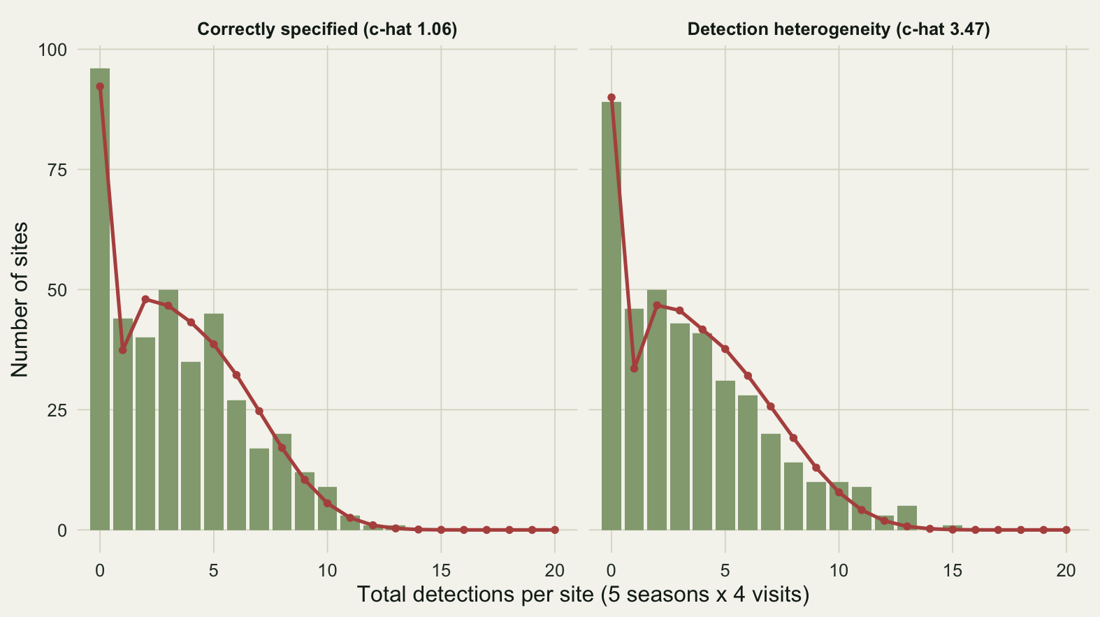
The check compares the observed distribution of total detections per site (a count from zero to twenty here) against the distribution the fitted model predicts. Because detection totals summarise the encounter histories, unmodelled heterogeneity shows up as over-dispersion: too many sites in both shoulders of the distribution, the hard-to-detect sites bunching at one and two detections and the easy ones spilling into the upper range around ten to thirteen, with a deficit in between. The zero cell itself is not the tell: a constant-detection fit reproduces the number of never-detected sites without trouble, so the misfit has to be looked for further along the axis. The expected distribution follows exactly from the forward algorithm, summed over every possible count history, so no simulation is needed to get it.
```{r}
#| label: statistic
exact_dist <- function(pr) {                 # exact P(total detections = j), j = 0..M
  ph <- exp(fwd_ll(Hgrid, pr, K)); agg <- tapply(ph, tot_grid, sum)
  out <- numeric(M + 1); out[as.integer(names(agg)) + 1] <- agg; out
}
X2 <- function(tot, E) {                      # Pearson statistic on the total-detection table
  O <- tabulate(tot + 1, nbins = M + 1); k <- E > 0.5   # tiny cells pooled into one
  sum((O[k] - E[k])^2 / E[k]) + (sum(O[!k]) - sum(E[!k]))^2 / sum(E[!k])
}
round(c(exact_dist_sums_to = sum(exact_dist(c(0.5, 0.2, 0.25, 0.35)))), 3)
```
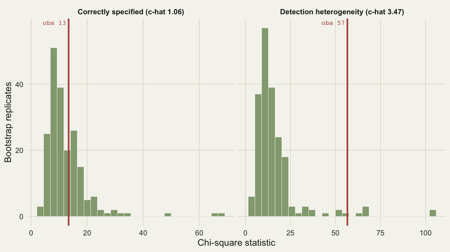
The Pearson statistic is not chi-square distributed here (the cells are sparse and the parameters were estimated), so its reference distribution comes from a parametric bootstrap: simulate a data set from the fitted model, refit it, recompute the statistic, and repeat. The ratio of the observed statistic to the average bootstrap statistic is the overdispersion factor `c-hat`, one when the model fits and larger when it does not.
```{r}
#| label: gof
gof <- function(d, seed, Bb = 200) {
  pr <- plogis(fitfun(d)$par); Eo <- exact_dist(pr) * R
  x2o <- X2(rowSums(d), Eo)
  set.seed(seed); x2b <- numeric(Bb)
  for (b in 1:Bb) {
    db <- gen(rep(pr[4], R), ps = pr[1], ga = pr[2], ep = pr[3])   # simulate from the fit
    fb <- plogis(fitfun(db)$par)
    x2b[b] <- X2(rowSums(db), exact_dist(fb) * R)
  }
  list(pr = pr, Eo = Eo, Oobs = tabulate(rowSums(d) + 1, nbins = M + 1),
       x2o = x2o, x2b = x2b, chat = x2o / mean(x2b), p = (1 + sum(x2b >= x2o)) / (Bb + 1))
}
gA <- gof(dA, seed = 107); gB <- gof(dB, seed = 506)
round(c(chat_homogeneous = gA$chat, p_homogeneous = gA$p,
        chat_heterogeneous = gB$chat, p_heterogeneous = gB$p), 3)
```
The correctly specified model has a `c-hat` of 1.13 and a bootstrap p-value of 0.33: the observed statistic sits comfortably among the values the model itself produces, and there is no evidence of lack of fit. The heterogeneous model has a `c-hat` of 3.49 and a p-value of 0.005. The observed statistic is more than three times the bootstrap average, which means the real data are far more spread out than a constant-detection model can account for.
```{r}
#| label: fig-total-dist
#| fig-cap: "Observed distribution of total detections per site (bars) against the fitted constant-detection expectation (line). Under heterogeneity the observed counts overload both shoulders and fall short in the middle."
#| fig-alt: "Two panels of bar charts with an overlaid expected line. In the correctly specified panel bars and line agree. In the heterogeneity panel the bars rise above the line just above zero and again from about ten to thirteen detections, and fall below it in between; both panels are empty above fifteen."
#| fig-width: 8.2
#| fig-height: 4.6
suppressMessages({library(ggplot2); library(dplyr); library(tidyr)})
theme_te <- function(bs = 12) theme_minimal(base_size = bs) + theme(
  plot.background = element_rect(fill = "#f5f4ee", colour = NA),
  panel.background = element_rect(fill = "#f5f4ee", colour = NA),
  panel.grid.major = element_line(colour = "#dad9ca", linewidth = 0.3),
  panel.grid.minor = element_blank(),
  axis.text = element_text(colour = "#2c3a31"), axis.title = element_text(colour = "#16241d"),
  plot.title = element_text(colour = "#16241d", face = "bold"),
  plot.subtitle = element_text(colour = "#46604a"),
  legend.position = "top", strip.text = element_text(colour = "#16241d", face = "bold"))

pA <- sprintf("Correctly specified (c-hat %.2f)", gA$chat)
pB <- sprintf("Detection heterogeneity (c-hat %.2f)", gB$chat)
mk <- function(g, lab) bind_rows(
  data.frame(tot = 0:M, count = g$Oobs, kind = "Observed", panel = lab),
  data.frame(tot = 0:M, count = g$Eo,   kind = "Expected", panel = lab))
dd1 <- bind_rows(mk(gA, pA), mk(gB, pB)); dd1$panel <- factor(dd1$panel, levels = c(pA, pB))
ggplot(dd1, aes(tot, count)) +
  geom_col(data = subset(dd1, kind == "Observed"), fill = "#93a87f", width = 0.85) +
  geom_line(data = subset(dd1, kind == "Expected"), aes(group = 1), colour = "#b5534e", linewidth = 0.9) +
  geom_point(data = subset(dd1, kind == "Expected"), colour = "#b5534e", size = 1.3) +
  facet_wrap(~panel) + coord_cartesian(xlim = c(0, M)) +
  labs(x = "Total detections per site (5 seasons x 4 visits)", y = "Number of sites") +
  theme_te()
```
The left panel shows the model reproducing its own data; bars and line agree. The right panel shows the signature of heterogeneity: an excess of sites in both shoulders, just above zero and again from about ten detections upward, with a deficit in between. This is what a mixture of easy and hard sites produces and a single detection probability cannot. The zero cell itself is fitted almost exactly, so none of the evidence sits there; the misfit is in the shoulders.
```{r}
#| label: fig-bootstrap
#| fig-cap: "Bootstrap distribution of the fit statistic under each fitted model, with the observed value marked. Inside the cloud means the model fits; deep in the tail means it does not."
#| fig-alt: "Two histograms of bootstrap chi-square values. In the correctly specified panel the red observed line falls within the histogram. In the heterogeneity panel the observed line lies well to the right of every bootstrap value."
#| fig-width: 8.2
#| fig-height: 4.6
dd2 <- bind_rows(data.frame(x2 = gA$x2b, panel = pA), data.frame(x2 = gB$x2b, panel = pB))
dd2$panel <- factor(dd2$panel, levels = c(pA, pB))
vl <- data.frame(panel = factor(c(pA, pB), levels = c(pA, pB)), x2o = c(gA$x2o, gB$x2o))
ggplot(dd2, aes(x2)) +
  geom_histogram(bins = 28, fill = "#93a87f", colour = "#f5f4ee", linewidth = 0.2) +
  geom_vline(data = vl, aes(xintercept = x2o), colour = "#b5534e", linewidth = 1) +
  geom_text(data = vl, aes(x = x2o, y = Inf, label = sprintf("obs %.0f", x2o)),
            colour = "#b5534e", hjust = 1.1, vjust = 1.6, size = 3, family = "mono") +
  facet_wrap(~panel, scales = "free_x") +
  labs(x = "Chi-square statistic", y = "Bootstrap replicates") +
  theme_te()
```
## What a high c-hat asks of you
An overdispersion factor above one is a prompt, not a verdict on any single parameter. The direct fix is to model the heterogeneity you suspect: put a covariate on detection when one is available, as in [covariates in dynamic occupancy models](../dynamic-occupancy-covariates/), or move to a detection model with a random effect or a finite mixture of detection classes. Where no structure is available, the pragmatic route is a quasi-likelihood adjustment: multiply the standard errors by the square root of `c-hat` and rank models with QAIC, which widens the intervals to acknowledge the extra variation even though it does not remove the bias. What is not defensible is reporting the tight intervals from the unadjusted fit as though the check had passed.
This is the end of the dynamic occupancy series. The basic model separated [colonisation and extinction](../dynamic-occupancy-colonisation-extinction/) from detection, [covariates](../dynamic-occupancy-covariates/) turned the rates into ecology, the [derived quantities](../occupancy-turnover-and-equilibrium/) gave the trajectory and equilibrium, and this check guards against trusting any of it when the detection assumption fails.
## References
- MacKenzie, Bailey 2004. Journal of Agricultural, Biological, and Environmental Statistics 9(3):300-318 (10.1198/108571104X3361).
- MacKenzie, Nichols, Hines, Knutson, Franklin 2003. Ecology 84(8):2200-2207 (10.1890/02-3090).
- Kery, Royle 2021. Applied Hierarchical Modeling in Ecology, Volume 2. ISBN 978-0-12-809585-0.
- MacKenzie, Nichols, Royle, Pollock, Bailey, Hines 2018. Occupancy Estimation and Modeling, 2nd ed. ISBN 978-0-12-407197-1.
## Related tutorials
- [Dynamic occupancy: colonisation and extinction](../dynamic-occupancy-colonisation-extinction/)
- [Checking a metapopulation model](../checking-a-metapopulation-model/)
- [Neighbourhood colonisation and false jumps](../neighbourhood-colonisation-and-false-jumps/)
- [Checking multi-state models](../checking-multistate-models/)