Checking multi-state models

Reasonable estimates do not mean a model fits. A bootstrap goodness-of-fit test in base R exposes hidden memory a standard multi-state model quietly absorbs.

The last three posts fitted multi-state and multi-event models and read parameters off them. None asked the prior question: does the model fit at all? This matters because a misspecified multi-state model rarely announces itself. The estimates come back at plausible values, the optimiser converges, and nothing looks wrong, even when a core assumption is violated. The most common violation is the Markov assumption itself. The standard Arnason-Schwarz model assumes the next state depends only on the current one, but animals often carry memory: an individual that just arrived somewhere may be more likely to return where it came from. Pradel, Wintrebert and Gimenez (2003) built the reference goodness-of-fit test for exactly this model, and pointed to the memory model of Brownie and others (1993) as the biologically plausible alternative when the test fails.

This post builds a parametric bootstrap goodness-of-fit test in base R, then shows it doing its job: passing data that really are Markov and flagging data that carry memory the fitted model ignores.

library(ggplot2)

theme_te <- function(bs = 12) theme_minimal(base_size = bs) + theme(
  text = element_text(colour = "#2c3a31"),
  plot.title = element_text(colour = "#16241d", face = "bold", size = rel(1.05)),
  plot.subtitle = element_text(colour = "#5d6b61", size = rel(0.9)),
  axis.title = element_text(colour = "#46604a"), axis.text = element_text(colour = "#46604a"),
  panel.grid.major = element_line(colour = "#dad9ca", linewidth = 0.3),
  panel.grid.minor = element_blank(),
  plot.background = element_rect(fill = "#f5f4ee", colour = NA),
  panel.background = element_rect(fill = "#f5f4ee", colour = NA),
  strip.text = element_text(colour = "#16241d", face = "bold"),
  legend.position = "bottom", legend.title = element_blank())
forest <- "#275139"; brick <- "#b5534e"; ink <- "#16241d"; gold <- "#c9b458"

phi_t <- 0.78; psiAB_t <- 0.30; psiBA_t <- 0.30; p_t <- 0.65
k <- 9; nA0 <- 360; nB0 <- 340; N <- nA0 + nB0
init_state <- c(rep(1L, nA0), rep(2L, nB0))

Two data-generating processes

The first process is a clean two-state Markov chain. The second adds memory: when an animal has just switched sites, it is more likely to switch back, a return tendency the Markov model has no way to represent. A single parameter mem controls the effect, with mem of zero recovering the Markov case.

sim_ms <- function(mem, p, seed) {
  set.seed(seed)
  y <- matrix(1L, N, k)
  for (i in 1:N) {
    s <- init_state[i]; sprev <- s; y[i, 1] <- if (s == 1L) 2L else 3L
    for (t in 2:k) {
      if (s == 3L) { y[i, t] <- 1L; next }
      pAB <- psiAB_t; pBA <- psiBA_t
      if (sprev != s && sprev != 3L) {              # just switched: raise return
        if (s == 2L && sprev == 1L) pBA <- min(1, psiBA_t + mem)
        if (s == 1L && sprev == 2L) pAB <- min(1, psiAB_t + mem)
      }
      if (runif(1) >= phi_t) { sprev <- s; s <- 3L; y[i, t] <- 1L; next }
      ns <- if (s == 1L) sample.int(2, 1, prob = c(1 - pAB, pAB))
            else         sample.int(2, 1, prob = c(pBA, 1 - pBA))
      sprev <- s
      s <- c(1L, 2L)[ns]
      y[i, t] <- if (s == 1L) sample.int(3, 1, prob = c(1 - p, p, 0))
                 else         sample.int(3, 1, prob = c(1 - p, 0, p))
    }
  }
  y
}

The model we fit is the standard Markov multi-state model from the first post, with state-specific detection.

Gam <- function(psiAB, psiBA, phi) matrix(c(
  phi * (1 - psiAB), phi * psiAB,     1 - phi,
  phi * psiBA,       phi * (1 - psiBA), 1 - phi,
  0,                 0,                1), nrow = 3, byrow = TRUE)
nll_ms <- function(par, y) {
  phi <- plogis(par[1]); psiAB <- plogis(par[2]); psiBA <- plogis(par[3])
  pA <- plogis(par[4]); pB <- plogis(par[5]); G <- Gam(psiAB, psiBA, phi)
  Pm <- list(c(1 - pA, 1 - pB, 1), c(pA, 0, 0), c(0, pB, 0)); ll <- 0
  for (i in 1:N) {
    a <- rep(0, 3); a[init_state[i]] <- 1; lg <- 0
    for (t in 2:k) { a <- (a %*% G) * Pm[[y[i, t]]]; s <- sum(a)
      if (s <= 0) return(1e10); a <- a / s; lg <- lg + log(s) }
    ll <- ll + lg
  }
  -ll
}
start <- c(qlogis(0.7), qlogis(0.3), qlogis(0.3), qlogis(0.6), qlogis(0.6))
fit_ms <- function(y) plogis(optim(start, nll_ms, y = y, method = "BFGS",
                                  control = list(maxit = 600))$par)
sim_markov <- function(th, seed) {
  set.seed(seed); phi <- th[1]; psiAB <- th[2]; psiBA <- th[3]; pA <- th[4]; pB <- th[5]
  G <- Gam(psiAB, psiBA, phi); y <- matrix(1L, N, k)
  for (i in 1:N) {
    s <- init_state[i]; y[i, 1] <- if (s == 1L) 2L else 3L
    for (t in 2:k) { s <- sample.int(3, 1, prob = G[s, ])
      if (s == 1L) y[i, t] <- sample.int(3, 1, prob = c(1 - pA, pA, 0))
      else if (s == 2L) y[i, t] <- sample.int(3, 1, prob = c(1 - pB, 0, pB)) }
  }
  y
}

A discrepancy that memory disturbs

A goodness-of-fit test needs a statistic that the assumption controls. Memory shows up as reversals, so we measure the reversal rate: among animals seen on three consecutive occasions where the first two states differ, how often does the third occasion return to the first state. Under a Markov model this is fixed by the transition probabilities; memory pushes it up.

Tstat <- function(y) {
  rev <- 0; sw <- 0
  for (i in 1:nrow(y)) {
    obs <- which(y[i, ] != 1L)
    if (length(obs) < 3) next
    st <- ifelse(y[i, obs] == 2L, 1L, 2L)
    for (j in 1:(length(obs) - 2)) {
      if (obs[j + 1] == obs[j] + 1 && obs[j + 2] == obs[j] + 2) {
        if (st[j] != st[j + 1]) { sw <- sw + 1; if (st[j + 2] == st[j]) rev <- rev + 1 }
      }
    }
  }
  if (sw == 0) return(NA); rev / sw
}
run_gof <- function(y, B = 200) {
  th <- fit_ms(y); Tobs <- Tstat(y); Tboot <- numeric(B)
  for (b in 1:B) Tboot[b] <- Tstat(sim_markov(th, seed = 9000 + b))
  Tboot <- Tboot[!is.na(Tboot)]
  list(Tobs = Tobs, Tboot = Tboot,
       pval = (1 + sum(Tboot >= Tobs)) / (1 + length(Tboot)), theta = th)
}

The test fits the Markov model, then simulates many data sets from the fitted model, recomputing the statistic each time to build its distribution under the assumption that the model is correct. If the observed value sits deep in the tail, the assumption is doubtful.

yM <- sim_ms(0.0, p_t, 138)                     # well specified
gofM <- run_gof(yM, B = 200)
yMem <- sim_ms(0.22, p_t, 138)                  # memory in the data
gofMem <- run_gof(yMem, B = 200)
data.frame(
  data = c("Markov", "Memory"),
  phi = c(round(gofM$theta[1], 3), round(gofMem$theta[1], 3)),
  psiAB = c(round(gofM$theta[2], 3), round(gofMem$theta[2], 3)),
  T_obs = c(round(gofM$Tobs, 3), round(gofMem$Tobs, 3)),
  boot_mean = c(round(mean(gofM$Tboot), 3), round(mean(gofMem$Tboot), 3)),
  gof_p = c(round(gofM$pval, 3), round(gofMem$pval, 3)))

    data   phi psiAB T_obs boot_mean gof_p
1 Markov 0.796 0.288 0.336     0.299 0.159
2 Memory 0.796 0.362 0.556     0.344 0.005

The parameter estimates give no warning. Both fits return survival near 0.8 and transitions in a believable range; read on their own they look fine. The goodness-of-fit test tells them apart. On the Markov data the observed reversal rate of 0.336 sits close to its bootstrap mean of 0.299, giving a p-value of 0.159: no evidence of misfit. On the memory data the observed reversal rate of 0.556 lies far above the bootstrap mean of 0.344, and no bootstrap sample reaches it, giving the smallest p-value 200 replicates can produce, 0.005: clear misfit.

bd <- rbind(
  data.frame(case = "Well-specified (Markov data)", T = gofM$Tboot),
  data.frame(case = "Misspecified (memory in data)", T = gofMem$Tboot))
bd$case <- factor(bd$case, levels = c("Well-specified (Markov data)", "Misspecified (memory in data)"))
obs <- data.frame(
  case = factor(c("Well-specified (Markov data)", "Misspecified (memory in data)"), levels = levels(bd$case)),
  Tobs = c(gofM$Tobs, gofMem$Tobs),
  lab = c(paste0("observed = ", round(gofM$Tobs, 3), "\np = ", round(gofM$pval, 3)),
          paste0("observed = ", round(gofMem$Tobs, 3), "\np = ", round(gofMem$pval, 3))),
  hj = c(-0.06, 1.06))
ggplot(bd, aes(T)) +
  geom_histogram(aes(y = after_stat(density)), bins = 26, fill = forest, alpha = 0.55, colour = NA) +
  geom_vline(data = obs, aes(xintercept = Tobs), colour = brick, linewidth = 1.1) +
  geom_text(data = obs, aes(x = Tobs, y = Inf, label = lab, hjust = hj), colour = ink, size = 3.3, vjust = 1.4) +
  facet_wrap(~case) +
  labs(title = "A goodness-of-fit test catches what estimates hide",
       subtitle = "Bootstrap distribution of the reversal statistic under the fitted Markov model; red is the observed value",
       x = "Reversal rate under the fitted model", y = "Density") +
  theme_te() + coord_cartesian(xlim = c(0.2, 0.62))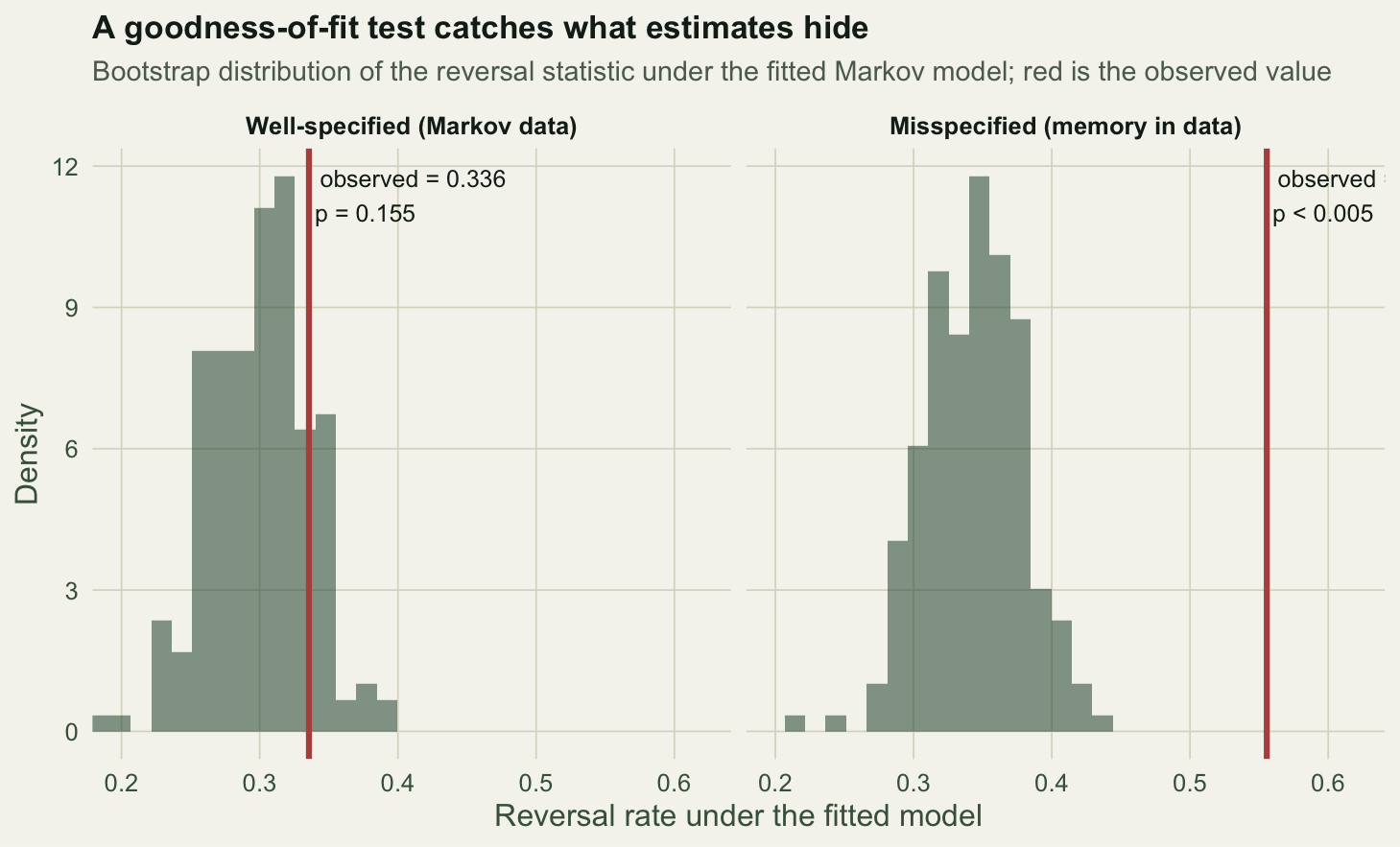

Figure 1: The estimates looked plausible in both cases. The reversal statistic is what separates them: on the memory data it lands beyond anything the fitted Markov model produces.

Sensitivity to the size of the problem

A test that only fires at one memory strength would not be much use. Sweeping mem upward shows the observed statistic climbing steadily out of the Markov null band, so the test detects memory across a range and, at mem of zero, correctly stays inside the band.

mem_grid <- c(0, 0.05, 0.10, 0.15, 0.20, 0.25)
R_rep <- 8
Tsweep <- sapply(mem_grid, function(mm)
  mean(sapply(1:R_rep, function(r) Tstat(sim_ms(mm, p_t, 1380 + r))), na.rm = TRUE))
null_lo <- as.numeric(quantile(gofM$Tboot, 0.025))
null_hi <- as.numeric(quantile(gofM$Tboot, 0.975))
data.frame(mem = mem_grid, T_obs = round(Tsweep, 3))

   mem T_obs
1 0.00 0.328
2 0.05 0.389
3 0.10 0.434
4 0.15 0.484
5 0.20 0.488
6 0.25 0.532

With no memory the observed statistic is 0.328, inside the null band of 0.228 to 0.37. By a memory strength of 0.25 it has risen to 0.532, well outside it.

sw <- data.frame(mem = mem_grid, Tobs = Tsweep)
ggplot(sw, aes(mem, Tobs)) +
  annotate("rect", xmin = -Inf, xmax = Inf, ymin = null_lo, ymax = null_hi, fill = gold, alpha = 0.25) +
  geom_hline(yintercept = mean(gofM$Tboot), linetype = "dashed", colour = "#7a6f2e", linewidth = 0.4) +
  annotate("text", x = 0.252, y = null_hi, label = "Markov null (95%)", colour = "#7a6f2e", size = 3.5, hjust = 1, vjust = -0.5) +
  geom_line(linewidth = 1, colour = brick) + geom_point(size = 2.8, colour = brick) +
  labs(title = "Test sensitivity rises with the strength of memory",
       subtitle = "Observed reversal rate leaves the Markov null band as second-order dependence grows",
       x = "Strength of state memory", y = "Observed reversal rate") + theme_te()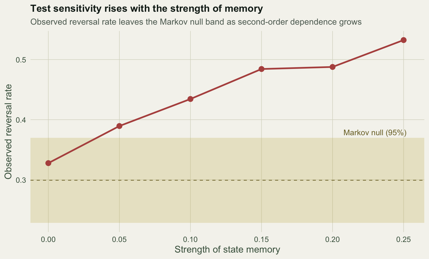

Figure 2: The test is not a one-point trick. The observed statistic climbs out of the null band as memory strengthens, and stays inside it when there is no memory to find.

What to remember

Plausible estimates are not evidence of fit. A multi-state model can absorb a violated assumption into slightly shifted parameters and give no outward sign, so fit has to be checked directly. A parametric bootstrap makes that check general: choose a statistic the assumption controls, simulate from the fitted model to get its null distribution, and see where the data fall. Here memory showed up as an excess of reversals, but the same recipe works for any discrepancy you can compute, from transience to overdispersion.

In practice you would not hand-roll every test. U-CARE and its R successor R2ucare implement the component tests of Pradel, Wintrebert and Gimenez (2003), which decompose overall fit into interpretable pieces, one sensitive to transience, another to exactly the memory effect shown here. When a test fails, the response is to enrich the model rather than ignore the warning: a memory model in the spirit of Brownie and others (1993), individual heterogeneity, or, if the misfit is mild overdispersion, a variance inflation factor to widen the intervals. A model worth trusting is one you have tried and failed to break.

This closes the group on multi-state and multi-event capture-recapture, from the basic model through transition estimation, uncertain states, and now fit.

References

Pradel R, Wintrebert CMA & Gimenez O 2003 Biometrics 59:43-53 (10.1111/1541-0420.00006)

Choquet R, Lebreton J-D, Gimenez O, Reboulet A-M & Pradel R 2009 Ecography 32:1071-1074 (10.1111/j.1600-0587.2009.05968.x)

Brownie C, Hines JE, Nichols JD, Pollock KH & Hestbeck JB 1993 Biometrics 49:1173-1187 (10.2307/2532259)

Lebreton J-D, Nichols JD, Barker RJ, Pradel R & Spendelow JA 2009 Advances in Ecological Research 41:87-173 (10.1016/S0065-2504(09)00403-6)

Gimenez O, Rossi V, Choquet R, Dehais C, Doris B, Varella H, Vila J-P & Pradel R 2007 Ecological Modelling 206:431-438 (10.1016/j.ecolmodel.2007.03.040)

Related tutorials

• Multi-state capture-recapture
• Estimating transition probabilities
• Multi-event models for uncertain states
• Checking a dynamic occupancy model