library(ggplot2)
theme_te <- function(bs = 12) theme_minimal(base_size = bs) + theme(
text = element_text(colour = "#2c3a31"),
plot.title = element_text(colour = "#16241d", face = "bold", size = rel(1.05)),
plot.subtitle = element_text(colour = "#5d6b61", size = rel(0.9)),
axis.title = element_text(colour = "#46604a"),
axis.text = element_text(colour = "#46604a"),
panel.grid.major = element_line(colour = "#dad9ca", linewidth = 0.3),
panel.grid.minor = element_blank(),
plot.background = element_rect(fill = "#f5f4ee", colour = NA),
panel.background = element_rect(fill = "#f5f4ee", colour = NA),
legend.position = "bottom", legend.title = element_blank())
ink <- "#16241d"; forest <- "#275139"; gold <- "#c9b458"; brick <- "#b5534e"Multi-state capture-recapture
R
capture-recapture
population dynamics
ecology tutorial
Fit an Arnason-Schwarz model by hand: state-specific survival, movement between states and state-specific detection, using a hidden Markov likelihood in base R.
A Cormack-Jolly-Seber model tracks one thing: is an animal alive or dead. Real study animals do more than that. They move between breeding sites, switch reproductive states, grow through size classes, or gain and lose disease status. If survival and detection differ by state, and animals move between states, a single survival estimate hides all of it.
The multi-state model (Arnason 1973; Schwarz, Schweigert and Arnason 1993; Brownie and others 1993) adds a state dimension to capture-recapture. Each individual occupies one of several live states at each occasion, survives with a state-specific probability, may move to another state, and is detected with a state-specific probability. This post fits the two-state case by hand, using the fact that a multi-state model is a hidden Markov model with an extra “dead” state.
The model
Consider two sites, A and B, and a marked animal seen once per year over several occasions. Three things vary by state:
- survival
phi_A,phi_B: the probability of surviving from one occasion to the next, given the current site; - movement
psi_AB,psi_BA: among survivors, the probability of moving to the other site; - detection
p_A,p_B: the probability of being seen, given the animal is alive and at that site.
The latent state at each occasion is one of alive-at-A, alive-at-B, or dead. The state process is a Markov chain with transition matrix
        to A              to B              dead
from A  phi_A (1-psi_AB)  phi_A psi_AB      1-phi_A
from B  phi_B psi_BA      phi_B (1-psi_BA)  1-phi_B
dead    0                 0                 1
Detection sits on top: an animal alive at A is seen at A with probability p_A, an animal alive at B is seen at B with probability p_B, and a dead animal is never seen. The observed history uses three codes at each occasion: not seen, seen at A, or seen at B.
Simulating known truth
Two sites with different survival (A is the better site), moderate movement, and different detection (A is easier to survey). We mark animals at both sites on the first occasion and follow them across the study.
phiA_t <- 0.75; phiB_t <- 0.60      # state-specific survival
psiAB_t <- 0.25; psiBA_t <- 0.15    # movement A->B and B->A
pA_t <- 0.55; pB_t <- 0.45          # state-specific detection
k <- 8                               # occasions
nA0 <- 260; nB0 <- 200               # initial marks per state
N <- nA0 + nB0

# state process (1 = alive-A, 2 = alive-B, 3 = dead); rows = from, cols = to
Gam <- function(phiA, phiB, psiAB, psiBA) matrix(c(
  phiA * (1 - psiAB), phiA * psiAB,     1 - phiA,
  phiB * psiBA,       phiB * (1 - psiBA), 1 - phiB,
  0,                  0,                1), nrow = 3, byrow = TRUE)
G_true <- Gam(phiA_t, phiB_t, psiAB_t, psiBA_t)
init_state <- c(rep(1L, nA0), rep(2L, nB0))
We mark 260 animals at A and 200 at B, and follow them for 8 occasions.
set.seed(135)
z <- matrix(0L, N, k)                # true latent state
y <- matrix(1L, N, k)                # observed event (1 = not seen)
for (i in 1:N) {
  z[i, 1] <- init_state[i]
  y[i, 1] <- if (z[i, 1] == 1L) 2L else 3L    # seen in its state when marked
  for (t in 2:k) {
    z[i, t] <- sample.int(3, 1, prob = G_true[z[i, t - 1], ])
    if (z[i, t] == 1L)      y[i, t] <- sample.int(3, 1, prob = c(1 - pA_t, pA_t, 0))
    else if (z[i, t] == 2L) y[i, t] <- sample.int(3, 1, prob = c(1 - pB_t, 0, pB_t))
    else                    y[i, t] <- 1L
  }
}
n_reseen <- sum(rowSums(y > 1L) > 1)
n_events <- sum(y > 1L)
Of 460 marked animals, 255 are seen again at least once, giving 973 detections in total.
The forward likelihood
The likelihood of one capture history is the probability of the observed events under the state process. Because the latent state is hidden, we sum over all state paths using the forward algorithm: start from the known state at first capture, and at each occasion multiply by the transition matrix and then by the detection probabilities for the observed event. Scaling at each step keeps the recursion from underflowing.
nll <- function(par) {
  phiA <- plogis(par[1]); phiB <- plogis(par[2])
  psiAB <- plogis(par[3]); psiBA <- plogis(par[4])
  pA <- plogis(par[5]); pB <- plogis(par[6])
  G <- Gam(phiA, phiB, psiAB, psiBA)
  Pm <- list(c(1 - pA, 1 - pB, 1),   # event 1: not seen
             c(pA, 0, 0),            # event 2: seen at A
             c(0, pB, 0))            # event 3: seen at B
  ll <- 0
  for (i in 1:N) {
    a <- rep(0, 3); a[init_state[i]] <- 1     # known state at first capture
    lg <- 0
    for (t in 2:k) {
      a <- (a %*% G) * Pm[[y[i, t]]]
      s <- sum(a); if (s <= 0) return(1e10)
      a <- a / s; lg <- lg + log(s)
    }
    ll <- ll + lg
  }
  -ll
}

start <- c(qlogis(0.5), qlogis(0.5), qlogis(0.2), qlogis(0.2), qlogis(0.4), qlogis(0.4))
fit <- optim(start, nll, method = "BFGS", hessian = TRUE, control = list(maxit = 500))
stopifnot(fit$convergence == 0)   # check before inverting the Hessian
est <- plogis(fit$par)
V <- solve(fit$hessian)
se_logit <- sqrt(diag(V))
lo <- plogis(fit$par - 1.96 * se_logit)
hi <- plogis(fit$par + 1.96 * se_logit)
nm <- c("phiA", "phiB", "psiAB", "psiBA", "pA", "pB")
truth <- c(phiA_t, phiB_t, psiAB_t, psiBA_t, pA_t, pB_t)
data.frame(parameter = nm, truth = truth, estimate = round(est, 3),
           lower = round(lo, 3), upper = round(hi, 3),
           covered = truth >= lo & truth <= hi)
parameter truth estimate lower upper covered
1 phiA 0.75 0.766 0.717 0.809 TRUE
2 phiB 0.60 0.635 0.587 0.682 TRUE
3 psiAB 0.25 0.317 0.252 0.390 FALSE
4 psiBA 0.15 0.158 0.116 0.210 TRUE
5 pA 0.55 0.623 0.532 0.707 TRUE
6 pB 0.45 0.445 0.369 0.524 TRUEThe model separates survival at A (0.766) from survival at B (0.635), and detection at A (0.623) from detection at B (0.445). 5 of the six confidence intervals cover the truth. The movement estimate psi_AB is 0.317, against a true 0.25. One realisation cannot separate sampling variation from bias, so we check that below.
What the naive analysis gets wrong
A tempting shortcut is to count the transitions you actually saw: of the animals detected at A on one occasion and detected again on the next, what fraction were at B. This ignores the states you missed through non-detection, and it is distorted by the difference in detection between sites.
nAA <- sum(y[, -k] == 2L & y[, -1] == 2L); nAB <- sum(y[, -k] == 2L & y[, -1] == 3L)
nBA <- sum(y[, -k] == 3L & y[, -1] == 2L); nBB <- sum(y[, -k] == 3L & y[, -1] == 3L)
naive_psiAB <- nAB / (nAA + nAB)
naive_psiBA <- nBA / (nBA + nBB)
c(naive_psiAB = round(naive_psiAB, 3), naive_psiBA = round(naive_psiBA, 3))
naive_psiAB naive_psiBA
0.239 0.200 # naive apparent return rate, ignoring state (a mix of survival and detection)
ret <- sum(vapply(1:N, function(i)
sum(vapply(1:(k - 1), function(t) y[i, t] > 1L && any(y[i, (t + 1):k] > 1L), logical(1))),
numeric(1)))
atrisk <- sum(y[, -k] > 1L)
round(ret / atrisk, 3)[1] 0.538The naive movement from B to A comes out at 0.2, against a true 0.15. Site B is harder to survey, so an animal that stays at B is often missed: the seen B-to-B pairs are under-represented, and that biases the apparent B-to-A rate upward. The naive apparent return rate, 0.538, pools across sites and mixes survival with detection.
lab <- c(phiA = "phi[A]", phiB = "phi[B]", psiAB = "psi[AB]",
         psiBA = "psi[BA]", pA = "p[A]", pB = "p[B]")
df <- data.frame(param = factor(nm, levels = rev(nm)), est = est,
                 lo = lo, hi = hi, truth = truth)
naive <- data.frame(param = factor(c("psiAB", "psiBA"), levels = rev(nm)),
                    val = c(naive_psiAB, naive_psiBA))
ggplot(df, aes(y = param)) +
  geom_segment(aes(x = lo, xend = hi, yend = param), colour = forest, linewidth = 1.1) +
  geom_point(aes(x = est), colour = forest, size = 3) +
  geom_point(aes(x = truth), colour = ink, shape = 124, size = 6) +
  geom_point(data = naive, aes(x = val), colour = brick, shape = 4, size = 3, stroke = 1.3) +
  scale_y_discrete(labels = function(x) parse(text = lab[x])) +
  labs(title = "Multi-state estimates and naive apparent transitions",
       subtitle = "Point and 95% CI (green), truth (dark bar), naive apparent transition (red cross)",
       x = "Probability", y = NULL) + theme_te()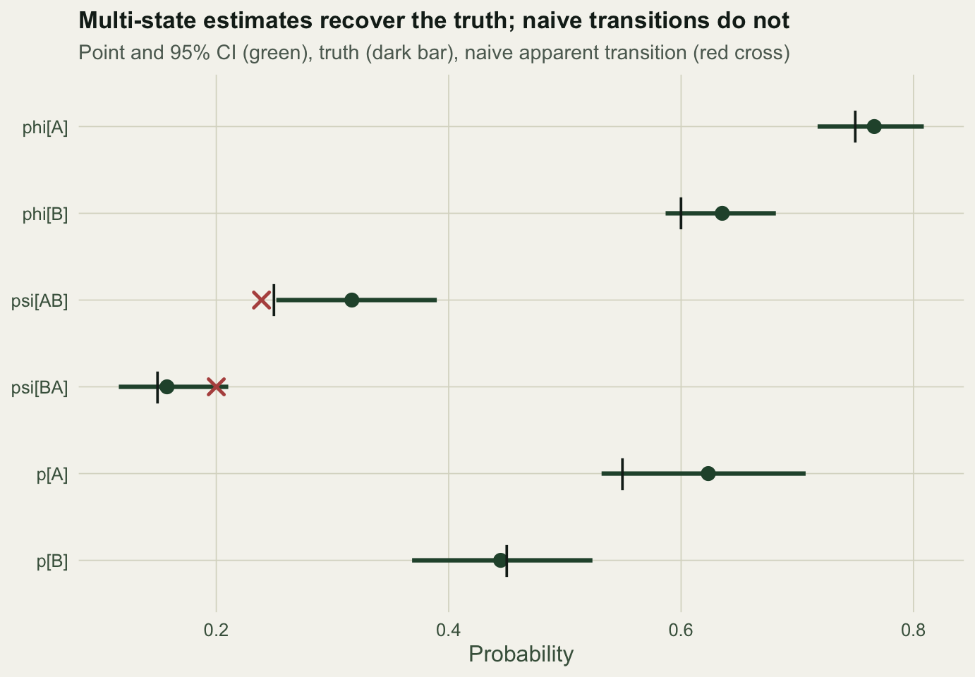
Is the estimator unbiased?
One data set cannot tell sampling variation apart from bias. To check, we simulate 40 fresh data sets from the same truth, refit each, and look at where the estimates land. If the estimator is unbiased, the estimates centre on the true values.
simulate_fit <- function(seed) {
  set.seed(seed)
  yy <- matrix(1L, N, k)
  for (i in 1:N) {
    s1 <- init_state[i]; yy[i, 1] <- if (s1 == 1L) 2L else 3L; st <- s1
    for (t in 2:k) {
      st <- sample.int(3, 1, prob = G_true[st, ])
      if (st == 1L)      yy[i, t] <- sample.int(3, 1, prob = c(1 - pA_t, pA_t, 0))
      else if (st == 2L) yy[i, t] <- sample.int(3, 1, prob = c(1 - pB_t, 0, pB_t))
    }
  }
  nll_s <- function(par) {
    phiA <- plogis(par[1]); phiB <- plogis(par[2]); psiAB <- plogis(par[3])
    psiBA <- plogis(par[4]); pA <- plogis(par[5]); pB <- plogis(par[6])
    G <- Gam(phiA, phiB, psiAB, psiBA)
    Pm <- list(c(1 - pA, 1 - pB, 1), c(pA, 0, 0), c(0, pB, 0)); ll <- 0
    for (i in 1:N) {
      a <- rep(0, 3); a[init_state[i]] <- 1; lg <- 0
      for (t in 2:k) { a <- (a %*% G) * Pm[[yy[i, t]]]; sm <- sum(a)
        if (sm <= 0) return(1e10); a <- a / sm; lg <- lg + log(sm) }
      ll <- ll + lg
    }
    -ll
  }
  plogis(optim(start, nll_s, method = "BFGS", control = list(maxit = 500))$par)
}

S <- 40
MC <- t(vapply(1000 + 1:S, simulate_fit, numeric(6)))
colnames(MC) <- nm
round(colMeans(MC) - truth, 4)   # Monte Carlo bias per parameter
phiA phiB psiAB psiBA pA pB
-0.0039 0.0031 0.0058 -0.0016 0.0105 0.0002 The row above prints, for each parameter, the average estimate across the replicates minus the truth. The practical message is that multi-state models estimate many parameters at once and are data-hungry: when detection is low or a state is rare, expect wide intervals, and check estimator behaviour by simulation before reading too much into any one number.
MCl <- stack(as.data.frame(MC)); names(MCl) <- c("value", "param")
MCl$param <- factor(MCl$param, levels = nm)
tr <- data.frame(param = factor(nm, levels = nm), truth = truth)
ggplot(MCl, aes(x = param, y = value)) +
  geom_boxplot(fill = "#e7e9df", colour = forest, outlier.size = 0.7, width = 0.55) +
  geom_point(data = tr, aes(x = param, y = truth), colour = brick, size = 3, shape = 18) +
  scale_x_discrete(labels = function(x) parse(text = lab[x])) +
  labs(title = "Where the estimates land across 40 replicate simulations",
       subtitle = "Boxplots of estimates across replicate simulations; red diamonds are true values",
       x = NULL, y = "Estimate") + theme_te()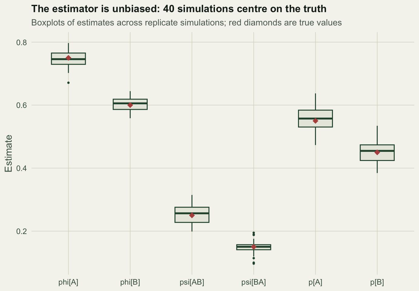
What to remember
A multi-state model separates state-specific survival, movement between states, and state-specific detection, all of which a single-state analysis pools together. The naive apparent-transition rate is biased whenever detection differs between states, because the states you miss are exactly the ones you cannot count. One structural caveat carries over from the CJS model: the survival and detection parameters in the final interval are only identifiable as a product, so treat the last occasion with care. And because the model fits many parameters from sparse detections, it needs plenty of data; a simulation check on estimator behaviour is cheap insurance.
The next post looks more closely at the movement parameters themselves, and at how state-specific detection can masquerade as movement if you are not careful.
References
Arnason AN 1973 Researches on Population Ecology 15:1-8 (10.1007/BF02510705)
Schwarz CJ, Schweigert JF & Arnason AN 1993 Biometrics 49:177-193 (10.2307/2532612)
Brownie C, Hines JE, Nichols JD, Pollock KH & Hestbeck JB 1993 Biometrics 49:1173-1187 (10.2307/2532259)
Hestbeck JB, Nichols JD & Malecki RA 1991 Ecology 72:523-533 (10.2307/2937193)
Lebreton J-D, Nichols JD, Barker RJ, Pradel R & Spendelow JA 2009 Advances in Ecological Research 41:87-173 (10.1016/S0065-2504(09)00403-6)
Gimenez O, Rossi V, Choquet R, Dehais C, Doris B, Varella H, Vila J-P & Pradel R 2007 Ecological Modelling 206:431-438 (10.1016/j.ecolmodel.2007.03.040)
Kery M & Schaub M 2012 Bayesian Population Analysis Using WinBUGS: A Hierarchical Perspective. Academic Press. ISBN 978-0-12-387020-9.