library(ggplot2)

theme_te <- function(bs = 12) theme_minimal(base_size = bs) + theme(
  text = element_text(colour = "#2c3a31"),
  plot.title = element_text(colour = "#16241d", face = "bold", size = rel(1.05)),
  plot.subtitle = element_text(colour = "#5d6b61", size = rel(0.9)),
  axis.title = element_text(colour = "#46604a"), axis.text = element_text(colour = "#46604a"),
  panel.grid.major = element_line(colour = "#dad9ca", linewidth = 0.3),
  panel.grid.minor = element_blank(),
  plot.background = element_rect(fill = "#f5f4ee", colour = NA),
  panel.background = element_rect(fill = "#f5f4ee", colour = NA),
  strip.text = element_text(colour = "#16241d", face = "bold"),
  legend.position = "bottom", legend.title = element_blank())
forest <- "#275139"; brick <- "#b5534e"; ink <- "#16241d"

# state process: latent 1 = alive-A, 2 = alive-B, 3 = dead
Gam <- function(psiAB, psiBA, phi) matrix(c(
  phi * (1 - psiAB), phi * psiAB,     1 - phi,
  phi * psiBA,       phi * (1 - psiBA), 1 - phi,
0, 0, 1), nrow = 3, byrow = TRUE)Multi-event models for uncertain states
R
capture-recapture
population dynamics
ecology tutorial
When the recorded state can be wrong, naive multi-state analysis mistakes error for movement. Multi-event models add an observation layer to recover them.
The two previous posts assumed that when you detect an animal, you know which state it is in. Often you do not. Sex can be ambiguous, breeding status hard to confirm, disease invisible without a test, a species easy to confuse with its neighbour. The state you write down is itself an observation, and observations can be wrong. When they are, a standard multi-state model reads the errors as movement: an animal seen as A one year and B the next looks like it moved, even if it never left.
Multi-event models, introduced by Pradel (2005), fix this by separating what is true from what is seen. Underneath sits the real state process, survival and transition as before. On top sits an event process: given the true state, what do you actually record? Because the event layer can misfire, the model can estimate how often it does and correct the transitions accordingly. This post builds a multi-event model in base R for the case that bites hardest, state misclassification.
The set-up
True movement is genuinely low: animals mostly stay put. Detection is moderate, and when an animal is detected its state is read correctly most of the time but misclassified with probability epsilon. An A read as B, or a B read as A, is our source of trouble.
phi_t <- 0.75; psiAB_t <- 0.15; psiBA_t <- 0.10   # low true movement
p_t <- 0.55; eps_t <- 0.15                          # detection and misclassification
k <- 8; nA0 <- 320; nB0 <- 280; N <- nA0 + nB0
init_state <- c(rep(1L, nA0), rep(2L, nB0))

# event: 1 = not seen, 2 = seen-as-A, 3 = seen-as-B
sim_me <- function(eps, p, seed) {
  set.seed(seed)
  y <- matrix(1L, N, k)
  for (i in 1:N) {
    s <- init_state[i]; y[i, 1] <- if (s == 1L) 2L else 3L   # state known at marking
    for (t in 2:k) {
      s <- sample.int(3, 1, prob = Gam(psiAB_t, psiBA_t, phi_t)[s, ])
      if (s == 1L)      y[i, t] <- sample.int(3, 1, prob = c(1 - p, p * (1 - eps), p * eps))
      else if (s == 2L) y[i, t] <- sample.int(3, 1, prob = c(1 - p, p * eps, p * (1 - eps)))
    }
  }
  y
}
The event layer is the only new machinery. Given the true state, the recorded event follows a small probability table: a detected A is seen as A with probability p(1 - eps) and as B with probability p * eps. The forward algorithm then sums over the unknown true states exactly as before.
# multi-event: par = phi, psiAB, psiBA, p, eps
nll_me <- function(par, y) {
  phi <- plogis(par[1]); psiAB <- plogis(par[2]); psiBA <- plogis(par[3])
  p <- plogis(par[4]); eps <- plogis(par[5])
  G <- Gam(psiAB, psiBA, phi)
  Pm <- list(c(1 - p, 1 - p, 1), c(p * (1 - eps), p * eps, 0), c(p * eps, p * (1 - eps), 0))
  ll <- 0
  for (i in 1:N) {
    a <- rep(0, 3); a[init_state[i]] <- 1; lg <- 0
    for (t in 2:k) { a <- (a %*% G) * Pm[[y[i, t]]]; s <- sum(a)
      if (s <= 0) return(1e10); a <- a / s; lg <- lg + log(s) }
    ll <- ll + lg
  }
  -ll
}
start_me <- c(qlogis(0.7), qlogis(0.2), qlogis(0.15), qlogis(0.5), qlogis(0.15))

# naive: take the recorded state as the truth (standard multi-state, eps ignored)
nll_naive <- function(par, y) {
  phi <- plogis(par[1]); psiAB <- plogis(par[2]); psiBA <- plogis(par[3])
  pA <- plogis(par[4]); pB <- plogis(par[5]); G <- Gam(psiAB, psiBA, phi)
  Pm <- list(c(1 - pA, 1 - pB, 1), c(pA, 0, 0), c(0, pB, 0)); ll <- 0
  for (i in 1:N) {
    a <- rep(0, 3); a[init_state[i]] <- 1; lg <- 0
    for (t in 2:k) { a <- (a %*% G) * Pm[[y[i, t]]]; s <- sum(a)
      if (s <= 0) return(1e10); a <- a / s; lg <- lg + log(s) }
    ll <- ll + lg
  }
  -ll
}
start_nv <- c(qlogis(0.7), qlogis(0.2), qlogis(0.15), qlogis(0.4), qlogis(0.4))
fit_naive <- function(y) plogis(optim(start_nv, nll_naive, y = y, method = "BFGS",
                                      control = list(maxit = 600))$par)
Fitting both models
We simulate one data set, fit the multi-event model with standard errors from the Hessian, and fit the naive model that trusts every recorded state.
y <- sim_me(eps_t, p_t, 137)
f <- optim(start_me, nll_me, y = y, method = "BFGS", hessian = TRUE, control = list(maxit = 700))
stopifnot(f$convergence == 0)   # check before inverting the Hessian
me <- plogis(f$par)
se <- sqrt(diag(solve(f$hessian)))
lo <- plogis(f$par - 1.96 * se); hi <- plogis(f$par + 1.96 * se)
nv <- fit_naive(y)
data.frame(param = c("phi", "psiAB", "psiBA", "p", "eps"),
           truth = c(phi_t, psiAB_t, psiBA_t, p_t, eps_t),
           multi_event = round(me, 3), lo = round(lo, 3), hi = round(hi, 3),
           naive = c(round(nv[1:3], 3), NA, NA))
param truth multi_event lo hi naive
1 phi 0.75 0.747 0.725 0.767 0.747
2 psiAB 0.15 0.150 0.107 0.207 0.265
3 psiBA 0.10 0.118 0.078 0.174 0.222
4 p 0.55 0.555 0.523 0.587 NA
5 eps 0.15 0.123 0.083 0.179 NAThe multi-event model recovers all five parameters, each true value inside its interval, including the misclassification rate itself at 0.123. The naive model gets survival right (0.747 against 0.75) but inflates both transitions badly: it reports movement from A to B of 0.265 against a truth of 0.15, and movement from B to A of 0.222 against 0.1. Nearly all of that apparent movement is misreading, not dispersal.
lab <- c(phi = "phi", psiAB = "psi[AB]", psiBA = "psi[BA]", p = "p", eps = "epsilon")
nm <- c("phi", "psiAB", "psiBA", "p", "eps")
est <- data.frame(param = factor(nm, levels = nm),
                  est = me, lo = lo, hi = hi, truth = c(phi_t, psiAB_t, psiBA_t, p_t, eps_t))
naive_df <- data.frame(param = factor(c("psiAB", "psiBA"), levels = nm), value = c(nv[2], nv[3]))
ggplot(est, aes(x = param)) +
  geom_point(aes(y = truth), shape = 95, size = 11, colour = ink) +
  geom_errorbar(aes(ymin = lo, ymax = hi), width = 0.16, colour = forest, linewidth = 0.8) +
  geom_point(aes(y = est, colour = "Multi-event MLE"), size = 3) +
  geom_point(data = naive_df, aes(y = value, colour = "Naive (states as truth)"), size = 3.4, shape = 17) +
  scale_x_discrete(labels = function(z) parse(text = lab[z])) +
  scale_colour_manual(values = c("Multi-event MLE" = forest, "Naive (states as truth)" = brick)) +
  labs(title = "Multi-event recovers every parameter; naive inflates movement",
       subtitle = "Points are estimates, bars are 95% CIs, dashes are the truth; naive transitions (triangles) sit far above",
       x = NULL, y = "Estimate") + theme_te()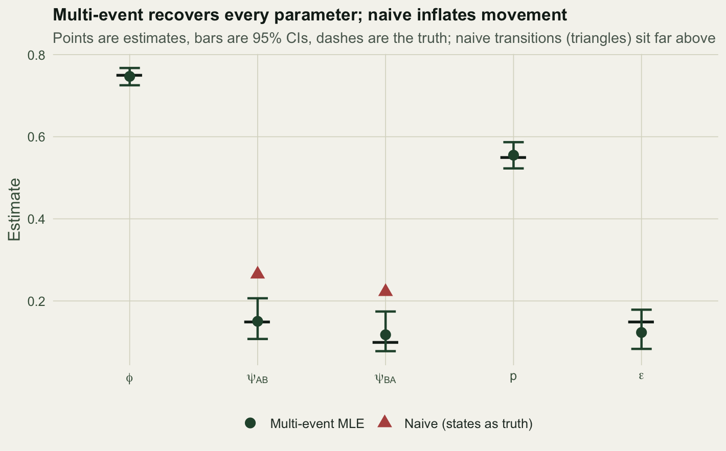
How the bias grows with error
To show this is systematic, we sweep the misclassification rate from zero upward and average several simulations at each level.
eps_grid <- c(0.00, 0.05, 0.10, 0.15, 0.20)
R_rep <- 10
rows <- list()
for (ep in eps_grid) {
  mAB <- mBA <- nAB <- nBA <- numeric(R_rep)
  for (r in 1:R_rep) {
    yy <- sim_me(ep, p_t, 1370 + r)
    mm <- plogis(optim(start_me, nll_me, y = yy, method = "BFGS", control = list(maxit = 700))$par)
    nnv <- fit_naive(yy)
    mAB[r] <- mm[2]; mBA[r] <- mm[3]; nAB[r] <- nnv[2]; nBA[r] <- nnv[3]
  }
  rows[[length(rows) + 1]] <- data.frame(eps = ep,
    psiAB_me = mean(mAB), psiBA_me = mean(mBA),
    psiAB_naive = mean(nAB), psiBA_naive = mean(nBA))
}
tab <- do.call(rbind, rows)
round(tab, 3)
eps psiAB_me psiBA_me psiAB_naive psiBA_naive
1 0.00 0.153 0.098 0.153 0.101
2 0.05 0.157 0.101 0.201 0.150
3 0.10 0.159 0.102 0.247 0.198
4 0.15 0.164 0.106 0.296 0.250
5 0.20 0.162 0.108 0.325 0.299At eps of zero the two models agree and both sit on the truth: with no misclassification, trusting the states is fine. As eps rises, the naive estimate of psi_AB climbs from 0.153 to 0.325, and psi_BA from 0.101 to 0.299, while the multi-event estimates hold near the true 0.15 and 0.1 throughout.
long <- rbind(
  data.frame(eps = tab$eps, param = "psi[AB]", method = "Naive", value = tab$psiAB_naive),
  data.frame(eps = tab$eps, param = "psi[AB]", method = "Multi-event", value = tab$psiAB_me),
  data.frame(eps = tab$eps, param = "psi[BA]", method = "Naive", value = tab$psiBA_naive),
  data.frame(eps = tab$eps, param = "psi[BA]", method = "Multi-event", value = tab$psiBA_me))
tru <- data.frame(param = c("psi[AB]", "psi[BA]"), truth = c(psiAB_t, psiBA_t))
ggplot(long, aes(eps, value, colour = method)) +
  geom_hline(data = tru, aes(yintercept = truth), linetype = "dashed", colour = ink, linewidth = 0.5) +
  geom_line(linewidth = 1) + geom_point(size = 2.6) +
  facet_wrap(~param, labeller = label_parsed) +
  scale_colour_manual(values = c("Multi-event" = forest, "Naive" = brick)) +
  labs(title = "Misclassification inflates apparent movement",
       subtitle = "As the misclassification rate rises, naive transitions climb; multi-event stays on the truth (dashed)",
       x = "Misclassification rate (epsilon)", y = "Estimated transition probability") + theme_te()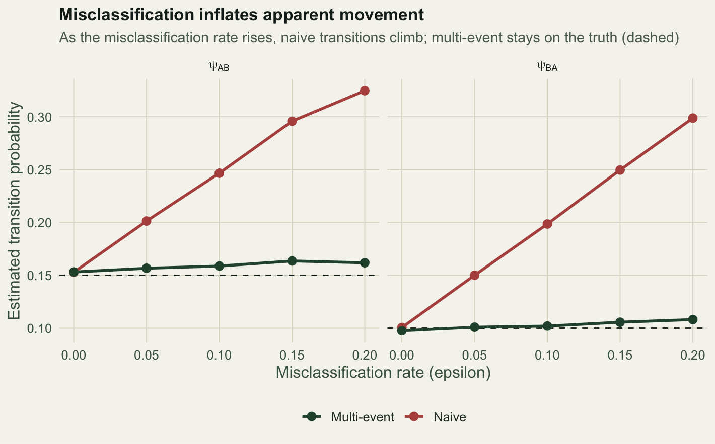
What to remember
When the recorded state can be wrong, misclassification masquerades as movement, and the naive transition estimate inflates in proportion to the error. The multi-event model separates the true state process from the observation process, estimates the misclassification rate directly, and returns the transitions to their true, lower values. Kendall, Hines and Nichols (2003) met the same problem in Florida manatees, with the bias running the other way: a female whose calf goes unseen is recorded as a non-breeder, so the conditional breeding probability came out at 0.31 when misclassification was ignored and 0.61 once it was accounted for, a difference large enough to change the demographic conclusion.
Two cautions. First, separating misclassification from real movement leans on information in the pattern of histories: a state that flickers back and forth looks like error, one that switches and stays looks like a transition. Weak data, few occasions, or very high error rates make the two hard to tell apart, and the extra parameter needs the sample size to support it. Second, a common field remedy is to gather repeat observations within a short closed window, several secondary samples per primary occasion as Kendall and others did, so that a truly static state can be confirmed against error. If your recorded states could be wrong, model the error rather than trusting the labels.
The final post in this group asks how you would know your multi-state or multi-event model fits at all, and what to do when it does not.
References
Pradel R 2005 Biometrics 61:442-447 (10.1111/j.1541-0420.2005.00318.x)
Kendall WL, Hines JE, Nichols JD 2003 Ecology 84:1058-1066 (10.1890/0012-9658(2003)084[1058:AMCMFM]2.0.CO;2)
Conn PB, Cooch EG 2009 Journal of Applied Ecology 46:486-492 (10.1111/j.1365-2664.2008.01597.x)
Gimenez O, Rossi V, Choquet R, Dehais C, Doris B, Varella H, Vila J-P, Pradel R 2007 Ecological Modelling 206:431-438 (10.1016/j.ecolmodel.2007.03.040)
Lebreton J-D, Nichols JD, Barker RJ, Pradel R, Spendelow JA 2009 Advances in Ecological Research 41:87-173 (10.1016/S0065-2504(09)00403-6)