Estimating transition probabilities

Movement between states is often the quantity of interest, but state-specific detection can masquerade as movement. A multi-state model separates the two.

In many studies the movement between states is the whole point. How often do animals switch breeding sites, move up a size class, or change disease status? Transition probabilities carry the ecology: the cost of reproduction, the strength of site fidelity, the speed of an epidemic. The multi-state model estimates them directly, but only if you respect a trap that catches the naive analysis: when detection differs between states, the states you fail to see distort the transitions you think you saw.

This post isolates that trap. We keep the two-site set-up from the previous post, hold detection at site A fixed, and let detection at site B fall. As the gap widens, we watch what happens to a naive transition estimate and to the multi-state estimate.

library(ggplot2)

theme_te <- function(bs = 12) theme_minimal(base_size = bs) + theme(
  text = element_text(colour = "#2c3a31"),
  plot.title = element_text(colour = "#16241d", face = "bold", size = rel(1.05)),
  plot.subtitle = element_text(colour = "#5d6b61", size = rel(0.9)),
  axis.title = element_text(colour = "#46604a"), axis.text = element_text(colour = "#46604a"),
  panel.grid.major = element_line(colour = "#dad9ca", linewidth = 0.3),
  panel.grid.minor = element_blank(),
  plot.background = element_rect(fill = "#f5f4ee", colour = NA),
  panel.background = element_rect(fill = "#f5f4ee", colour = NA),
  strip.text = element_text(colour = "#16241d", face = "bold"),
  legend.position = "bottom", legend.title = element_blank())
forest <- "#275139"; brick <- "#b5534e"; ink <- "#16241d"

# two sites; latent 1 = alive-A, 2 = alive-B, 3 = dead
Gam <- function(phiA, phiB, psiAB, psiBA) matrix(c(
  phiA * (1 - psiAB), phiA * psiAB,     1 - phiA,
  phiB * psiBA,       phiB * (1 - psiBA), 1 - phiB,
  0,                  0,                1), nrow = 3, byrow = TRUE)

The set-up

True survival, movement and detection at A are fixed. Detection at B is the knob we turn. We mark plenty of animals so that sampling noise is small and any drift we see is real.

phiA_t <- 0.72; phiB_t <- 0.62      # survival
psiAB_t <- 0.30; psiBA_t <- 0.20    # movement (the target)
pA_t <- 0.60                         # detection at A (fixed)
k <- 8; nA0 <- 320; nB0 <- 280; N <- nA0 + nB0
G_true <- Gam(phiA_t, phiB_t, psiAB_t, psiBA_t)
init_state <- c(rep(1L, nA0), rep(2L, nB0))
start <- c(qlogis(0.5), qlogis(0.5), qlogis(0.25), qlogis(0.25), qlogis(0.5), qlogis(0.4))

sim_data <- function(pB, seed) {
  set.seed(seed)
  y <- matrix(1L, N, k)
  for (i in 1:N) {
    s <- init_state[i]; y[i, 1] <- if (s == 1L) 2L else 3L
    for (t in 2:k) {
      s <- sample.int(3, 1, prob = G_true[s, ])
      if (s == 1L)      y[i, t] <- sample.int(3, 1, prob = c(1 - pA_t, pA_t, 0))
      else if (s == 2L) y[i, t] <- sample.int(3, 1, prob = c(1 - pB, 0, pB))
    }
  }
  y
}

The multi-state fit reuses the forward likelihood from the previous post.

mle_fit <- function(y) {
  nll <- function(par) {
    phiA <- plogis(par[1]); phiB <- plogis(par[2]); psiAB <- plogis(par[3])
    psiBA <- plogis(par[4]); pA <- plogis(par[5]); pB <- plogis(par[6])
    G <- Gam(phiA, phiB, psiAB, psiBA)
    Pm <- list(c(1 - pA, 1 - pB, 1), c(pA, 0, 0), c(0, pB, 0)); ll <- 0
    for (i in 1:N) {
      a <- rep(0, 3); a[init_state[i]] <- 1; lg <- 0
      for (t in 2:k) { a <- (a %*% G) * Pm[[y[i, t]]]; s <- sum(a)
        if (s <= 0) return(1e10); a <- a / s; lg <- lg + log(s) }
      ll <- ll + lg
    }
    -ll
  }
  plogis(optim(start, nll, method = "BFGS", control = list(maxit = 500))$par)
}

# naive: count only the transitions you actually saw on consecutive occasions
naive_psi <- function(y) {
  nAA <- sum(y[, -k] == 2L & y[, -1] == 2L); nAB <- sum(y[, -k] == 2L & y[, -1] == 3L)
  nBA <- sum(y[, -k] == 3L & y[, -1] == 2L); nBB <- sum(y[, -k] == 3L & y[, -1] == 3L)
  c(psiAB = nAB / (nAA + nAB), psiBA = nBA / (nBA + nBB))
}

Turning the detection knob

For each level of detection at B, we simulate several data sets, fit both estimators, and average. Averaging strips out sampling noise so the systematic pattern stands clear.

pB_grid <- c(0.60, 0.50, 0.40, 0.30, 0.20)
R_rep <- 12
rows <- list()
for (pB in pB_grid) {
  mm <- matrix(NA, R_rep, 2); nn <- matrix(NA, R_rep, 2)
  for (r in 1:R_rep) {
    y <- sim_data(pB, seed = 136 * 10 + r)
    mm[r, ] <- mle_fit(y)[3:4]; nn[r, ] <- naive_psi(y)
  }
  rows[[length(rows) + 1]] <- data.frame(
    gap = pA_t - pB, pB = pB,
    psiAB_naive = mean(nn[, 1]), psiBA_naive = mean(nn[, 2]),
    psiAB_mle = mean(mm[, 1]),   psiBA_mle = mean(mm[, 2]))
}
tab <- do.call(rbind, rows)
round(tab, 3)

  gap  pB psiAB_naive psiBA_naive psiAB_mle psiBA_mle
1 0.0 0.6       0.300       0.197     0.301     0.196
2 0.1 0.5       0.258       0.223     0.294     0.194
3 0.2 0.4       0.220       0.261     0.297     0.197
4 0.3 0.3       0.178       0.317     0.297     0.195
5 0.4 0.2       0.130       0.416     0.315     0.196

With no gap (p_B equal to p_A at 0.60), the naive estimate of psi_AB is 0.3, right on the true 0.30: high detection everywhere means few missed states. As the gap opens, the naive estimate of movement from A to B falls to 0.13 at a gap of 0.4, while the naive movement from B to A climbs to 0.416. The multi-state estimates barely move: psi_AB stays near 0.3 and psi_BA near 0.2 across the whole range.

The direction makes sense. When site B is under-surveyed, an animal that stays at B is often missed, so among the pairs you do see, B-to-B is under-counted and B-to-A looks inflated. The same missing B-detections make A-to-B moves vanish, deflating psi_AB. Detection has disguised itself as movement.

long <- rbind(
  data.frame(gap = tab$gap, param = "psi[AB]", method = "Naive", value = tab$psiAB_naive),
  data.frame(gap = tab$gap, param = "psi[AB]", method = "Multi-state", value = tab$psiAB_mle),
  data.frame(gap = tab$gap, param = "psi[BA]", method = "Naive", value = tab$psiBA_naive),
  data.frame(gap = tab$gap, param = "psi[BA]", method = "Multi-state", value = tab$psiBA_mle))
tru <- data.frame(param = c("psi[AB]", "psi[BA]"), truth = c(psiAB_t, psiBA_t))
ggplot(long, aes(gap, value, colour = method)) +
  geom_hline(data = tru, aes(yintercept = truth), linetype = "dashed", colour = ink, linewidth = 0.5) +
  geom_line(linewidth = 1) + geom_point(size = 2.6) +
  facet_wrap(~param, labeller = label_parsed) +
  scale_colour_manual(values = c("Multi-state" = forest, "Naive" = brick)) +
  labs(title = "State-specific detection makes naive transitions drift",
       subtitle = "As detection at B drops below A, the naive estimate leaves the truth (dashed)",
       x = "Detection gap (p_A minus p_B)", y = "Estimated transition probability") + theme_te()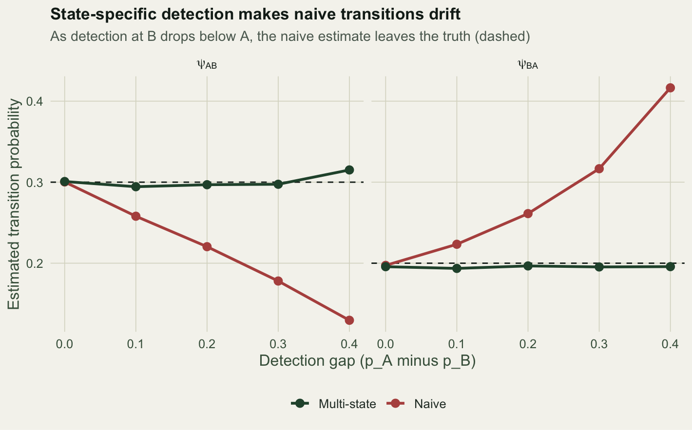

Figure 1

How bad is it at a realistic gap?

A detection gap of 0.3 is unremarkable in the field: one site with good access, one without. We simulate 30 data sets at that gap and compare the sampling distributions of the two estimators.

S <- 30
mcM <- matrix(NA, S, 2); mcN <- matrix(NA, S, 2)
for (s in 1:S) {
  ys <- sim_data(0.30, seed = 2000 + s)
  mcM[s, ] <- mle_fit(ys)[3:4]; mcN[s, ] <- naive_psi(ys)
}
rbind(multistate = round(colMeans(mcM), 3), naive = round(colMeans(mcN), 3))

            [,1]  [,2]
multistate 0.303 0.195
naive      0.179 0.331

The multi-state estimator centres on the truth (psi_AB 0.303, psi_BA 0.195 against 0.30 and 0.20). The naive estimator is off in both directions and stays off: more data would not fix it, because the bias is structural, not random.

mc <- rbind(
  data.frame(param = "psi[AB]", method = "Naive", value = mcN[, 1]),
  data.frame(param = "psi[AB]", method = "Multi-state", value = mcM[, 1]),
  data.frame(param = "psi[BA]", method = "Naive", value = mcN[, 2]),
  data.frame(param = "psi[BA]", method = "Multi-state", value = mcM[, 2]))
ggplot(mc, aes(x = method, y = value, fill = method)) +
  geom_boxplot(width = 0.5, colour = "#3a3a3a", outlier.size = 0.6) +
  geom_hline(data = tru, aes(yintercept = truth), linetype = "dashed", colour = ink, linewidth = 0.5) +
  facet_wrap(~param, labeller = label_parsed, scales = "free_y") +
  scale_fill_manual(values = c("Multi-state" = forest, "Naive" = brick)) +
  labs(title = "At a detection gap of 0.3, the naive estimate is systematically off",
       subtitle = "30 simulations; multi-state centres on the truth (dashed), naive does not",
       x = NULL, y = "Estimate") + theme_te() + theme(legend.position = "none")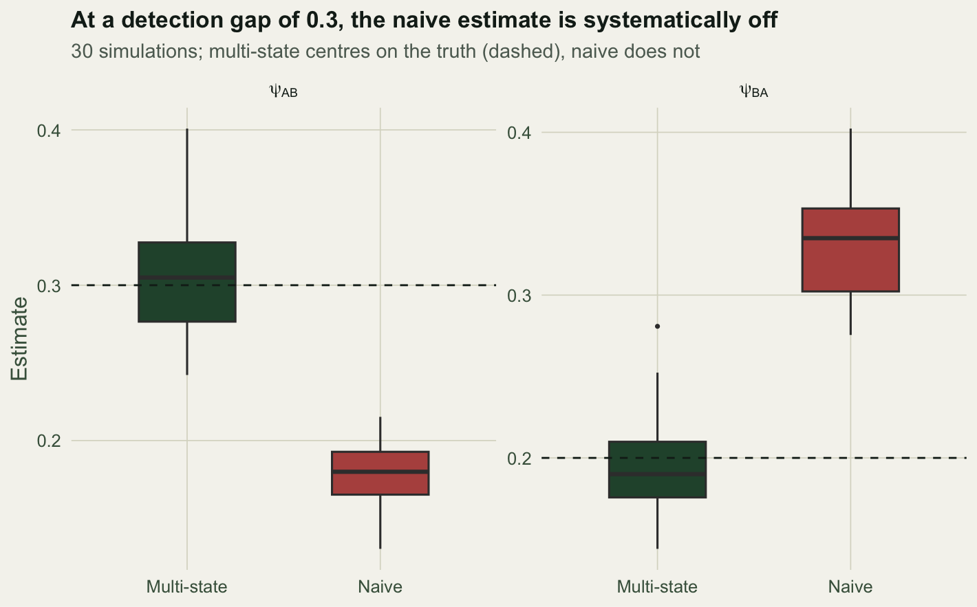

Figure 2

What to remember

State-specific detection biases the naive transition estimate, and the bias grows with the detection gap. When you undercount a state, animals that stay there look like they left, and animals that arrive there look like they never came. The multi-state model estimates detection and movement jointly, so it is unbiased across the whole range of gaps.

The practical warning is about interpretation. A naive analysis of the data above would report weaker fidelity at the poorly surveyed site, an ecological conclusion that is an artefact of the survey, not the biology. Nichols and others (1994) made exactly this point for breeding proportions: breeders and non-breeders are usually seen at different rates, so the multi-state framework is what lets you test for a cost of reproduction without confounding it with detection. If detection could plausibly differ between your states, estimate it; do not assume it away.

The next post goes one step further, to the case where you cannot even be sure which state an animal is in when you do see it.

References

Hestbeck, J.B., Nichols, J.D. & Malecki, R.A. (1991). Estimates of movement and site fidelity using mark-resight data of wintering Canada geese. Ecology, 72, 523-533. https://doi.org/10.2307/2937193

Brownie, C., Hines, J.E., Nichols, J.D., Pollock, K.H. & Hestbeck, J.B. (1993). Capture-recapture studies for multiple strata including non-Markovian transitions. Biometrics, 49, 1173-1187. https://doi.org/10.2307/2532259

Nichols, J.D., Hines, J.E., Pollock, K.H., Hinz, R.L. & Link, W.A. (1994). Estimating breeding proportions and testing hypotheses about costs of reproduction with capture-recapture data. Ecology, 75, 2052-2065. https://doi.org/10.2307/1941610

Lebreton, J.-D. & Pradel, R. (2002). Multistate recapture models: modelling incomplete individual histories. Journal of Applied Statistics, 29, 353-369. https://doi.org/10.1080/02664760120108638

Lebreton, J.-D., Nichols, J.D., Barker, R.J., Pradel, R. & Spendelow, J.A. (2009). Modeling individual animal histories with multistate capture-recapture models. Advances in Ecological Research, 41, 87-173. https://doi.org/10.1016/S0065-2504(09)00403-6

Kery, M. & Schaub, M. (2012). Bayesian Population Analysis Using WinBUGS: A Hierarchical Perspective. Academic Press. ISBN 978-0-12-387020-9.

Related tutorials

• Multi-state capture-recapture
• Multi-event models for uncertain states
• Checking multi-state models
• Cormack-Jolly-Seber survival

References

Hestbeck JB, Nichols JD, Malecki RA 1991 Ecology 72:523-533 (10.2307/2937193)