Cormack-Jolly-Seber survival models in R

Estimate apparent survival and recapture from open capture histories in R: build the m-array and fit a Cormack-Jolly-Seber model by maximum likelihood.

When survival is estimated from repeated captures of marked animals rather than from known fates, a return rate cannot be read off directly, because an animal that is not seen again might be dead or might simply have gone undetected. The Cormack-Jolly-Seber model separates those two possibilities. From capture histories it estimates apparent survival, the probability of surviving and staying in the study area between occasions, and recapture probability, the chance of detecting an animal that is present. This post reduces capture histories to an m-array and fits the constant model by maximum likelihood in base R with optim, recovering the survival and detection parameters that a naive return rate confounds. It is the open-population counterpart to the closed capture-recapture models, which estimate abundance when no births, deaths or movement occur during sampling.

From capture histories to an m-array

A capture history is a row of ones and zeros recording whether each marked animal was caught on each occasion. The efficient summary for a constant model is the m-array: for each release occasion, how many animals were released, and of those, at which later occasion each was next recaptured. The example is a study of 7 occasions with true apparent survival of 0.72 and recapture probability of 0.42.

library(ggplot2)
library(dplyr)
library(tidyr)

set.seed(519)
k <- 7; N <- 400
phi_true <- 0.72; p_true <- 0.42
alive <- matrix(0L, N, k); alive[, 1] <- 1L
for (t in 2:k) alive[, t] <- alive[, t - 1] * (runif(N) < phi_true)
capt <- matrix(0L, N, k)
capt[alive == 1] <- (runif(sum(alive == 1)) < p_true)
ch <- capt[rowSums(capt) > 0, , drop = FALSE]        # keep animals caught at least once
c(ever_caught = nrow(ch), total_captures = sum(ch), occasions = k)

   ever_caught total_captures      occasions 
           278            532              7 

Every capture before the final occasion is a release, and each release is followed either by a next recapture or by the animal never being seen again. Tallying those outcomes fills the m-array.

Rrel <- integer(k); m <- matrix(0L, k, k)
for (r in seq_len(nrow(ch))) {
  occ <- which(ch[r, ] == 1L)
  rel <- occ[occ < k]                                # captures at occasions 1..k-1
  Rrel[rel] <- Rrel[rel] + 1L
  if (length(occ) > 1)
    for (a in seq_len(length(occ) - 1)) m[occ[a], occ[a + 1]] <- m[occ[a], occ[a + 1]] + 1L
}
ma <- cbind(released = Rrel[1:(k - 1)], m[1:(k - 1), 2:k])
ma <- cbind(ma, never = Rrel[1:(k - 1)] - rowSums(m[1:(k - 1), 2:k]))
colnames(ma) <- c("released", paste0("recap_", 2:k), "never")
rownames(ma) <- paste0("release_", 1:(k - 1))
ma

          released recap_2 recap_3 recap_4 recap_5 recap_6 recap_7 never
release_1      155      51      27       7       2       2       0    66
release_2      133       0      43      19       4       2       1    64
release_3       94       0       0      22      15       3       4    50
release_4       58       0       0       0      21       4       0    33
release_5       48       0       0       0       0      14       4    30
release_6       26       0       0       0       0       0       9    17

Each row is a release cohort. Of the 155 animals released at the first occasion, 51 were next seen at occasion 2, 27 at occasion 3, a handful later, and 66 were never seen again. The recaptures decay across the row because each extra gap requires the animal to survive again and still be missed at every occasion in between.

msub <- m[1:(k - 1), 2:k]
dimnames(msub) <- list(release = paste0("occ ", 1:(k - 1)),
                       recapture = paste0("occ ", 2:k))
mm <- as.data.frame(as.table(msub))
names(mm) <- c("release", "recapture", "count")
mm$release   <- factor(mm$release,   levels = rev(paste0("occ ", 1:(k - 1))))
mm$recapture <- factor(mm$recapture, levels = paste0("occ ", 2:k))

ggplot(mm, aes(recapture, release, fill = count)) +
  geom_tile(colour = te_paper, linewidth = 1) +
  geom_text(aes(label = count), colour = te_ink, size = 3.1) +
  scale_fill_gradient(low = te_paper, high = te_forest) +
  labs(title = "The m-array of first recaptures",
       subtitle = "Counts concentrate just after release and fade with the gap",
       x = "Occasion of next recapture", y = "Release occasion") +
  theme_te() +
  theme(panel.grid.major = element_blank())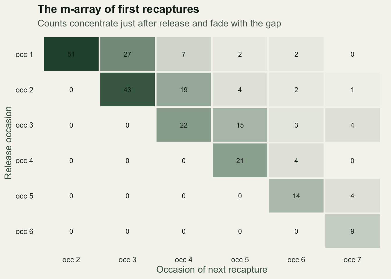

Figure 1: The m-array as a heatmap: rows are release cohorts, columns are the occasion of next recapture, and shading and labels give the counts.

The Cormack-Jolly-Seber likelihood

For the constant model each release cohort is a multinomial draw. An animal released at occasion i and next seen at occasion j must have survived every step from i to j and been missed at every occasion in between, then detected at j, which for constant parameters is survival to the power of the gap, times one-minus-detection for each missed occasion, times detection. The remaining probability, of never being seen again, closes each cohort. Summing the log multinomial across cohorts gives the log-likelihood, maximised on the logit scale so the parameters stay between zero and one.

negll <- function(par) {
  phi <- plogis(par[1]); p <- plogis(par[2]); ll <- 0
  for (i in 1:(k - 1)) {
    Ri <- Rrel[i]; if (Ri == 0) next
    seen <- 0
    for (j in (i + 1):k) {
      q <- phi^(j - i) * (1 - p)^(j - i - 1) * p       # first seen again at j
      if (m[i, j] > 0) ll <- ll + m[i, j] * log(q)
      seen <- seen + q
    }
    never <- Ri - sum(m[i, (i + 1):k])
    if (never > 0) ll <- ll + never * log(1 - seen)    # never seen again
  }
  -ll
}

fit <- optim(c(0, 0), negll, method = "BFGS", hessian = TRUE)
est <- plogis(fit$par)
se_logit <- sqrt(diag(solve(fit$hessian)))
se_prob <- se_logit * est * (1 - est)                  # delta method to the probability scale
ci <- t(sapply(1:2, function(i) plogis(fit$par[i] + c(-1.96, 1.96) * se_logit[i])))

data.frame(parameter = c("apparent survival (phi)", "recapture (p)"),
           estimate = round(est, 4), se = round(se_prob, 4),
           lower = round(ci[, 1], 3), upper = round(ci[, 2], 3),
           truth = c(phi_true, p_true))

                parameter estimate     se lower upper truth
1 apparent survival (phi)   0.7069 0.0216 0.663 0.747  0.72
2           recapture (p)   0.4494 0.0302 0.391 0.509  0.42

Apparent survival comes out at about 0.71 with a confidence interval from 0.66 to 0.75, and recapture at about 0.45 from 0.39 to 0.51, both close to the values that generated the data. The model has pulled two parameters out of the pattern of recaptures and gaps, using the fact that survival controls how many animals return at all while detection controls how quickly they reappear once they do.

ed <- data.frame(parameter = c("Apparent survival", "Recapture probability"),
                 est = est, lo = ci[, 1], hi = ci[, 2], truth = c(phi_true, p_true))

ggplot(ed, aes(est, parameter)) +
  geom_errorbarh(aes(xmin = lo, xmax = hi), height = 0.15, colour = te_forest, linewidth = 0.8) +
  geom_point(colour = te_forest, size = 2.6) +
  geom_point(aes(x = truth), colour = te_brick, shape = 4, size = 3, stroke = 1.1) +
  annotate("text", x = ed$truth[1], y = 1.28, label = "true", colour = te_brick, size = 3.0) +
  coord_cartesian(xlim = c(0.3, 0.8)) +
  labs(title = "Estimates recover the generating values",
       subtitle = "Points and intervals are the fitted estimates; crosses mark the truth",
       x = "Probability", y = NULL) +
  theme_te()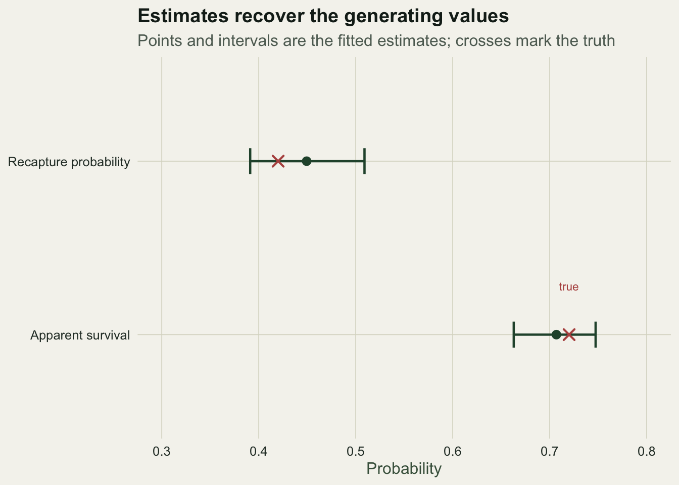

Figure 2: Cormack-Jolly-Seber estimates with 95 per cent confidence intervals against the true values (crosses).

Apparent survival, and what it does not include

Two cautions travel with these estimates. The first is that a raw return rate is not survival: here about 49 per cent of releases were ever seen again, a figure that blends mortality with imperfect detection and matches neither parameter. The second is in the word apparent. The model cannot tell a dead animal from one that survived but permanently left the study area, so apparent survival is the product of true survival and site fidelity, and it is a lower bound on true survival. A further structural point is that the last survival and last recapture are only ever seen multiplied together, so in a fully time-varying model they cannot be separated; the constant model sidesteps this by sharing one parameter across occasions.

Where to go next

The Cormack-Jolly-Seber model is the open-population sibling of the closed capture-recapture estimators, which count a fixed population, and it shares its by-hand likelihood machinery with the N-mixture model, where a latent count is summed out rather than a latent survival path. The apparent survival it returns is the same quantity a life table treats as known, so a capture study can feed the survival schedule of a matrix population model. Extending the constant model to time-varying or covariate-dependent survival follows the framework laid out by Lebreton and colleagues.

References

Cormack RM 1964. Biometrika 51(3-4):429-438 (10.1093/biomet/51.3-4.429).

Jolly GM 1965. Biometrika 52(1-2):225-247 (10.1093/biomet/52.1-2.225).

Seber GAF 1965. Biometrika 52(1-2):249-259 (10.1093/biomet/52.1-2.249).

Lebreton JD, Burnham KP, Clobert J, Anderson DR 1992. Ecological Monographs 62(1):67-118 (10.2307/2937171).

Related tutorials

• Closed-population capture-recapture in R
• N-mixture models for abundance
• Kaplan-Meier survival curves and the log-rank test
• Life tables and the population growth rate