library(ggplot2)

te_paper  <- "#f5f4ee"
te_ink    <- "#16241d"
te_body   <- "#2c3a31"
te_forest <- "#275139"
te_rust   <- "#b5534e"
te_gold   <- "#c9b458"
te_line   <- "#dad9ca"

theme_datasheet <- function() {
  theme_minimal(base_size = 12) +
    theme(plot.background  = element_rect(fill = te_paper, colour = NA),
          panel.background = element_rect(fill = te_paper, colour = NA),
          panel.grid.major = element_line(colour = te_line, linewidth = 0.3),
          panel.grid.minor = element_blank(),
          text             = element_text(colour = te_body),
          plot.title       = element_text(colour = te_ink, face = "bold"),
          plot.subtitle    = element_text(colour = te_body),
          axis.text        = element_text(colour = te_body))
}Joint live-dead models: survival or fidelity?
R
capture-recapture
survival analysis
population ecology
ecology tutorial
Apparent survival from a live-only capture-recapture model is true survival times site fidelity. Adding dead recoveries in R separates the two, exactly.
A ringing scheme hears about a marked bird in two ways. The first is a recapture: the bird is caught again at the colony, alive, and the ring is read. The second is a recovery: someone finds the bird dead, possibly hundreds of kilometres away, and posts the ring back. The two channels arrive in different columns of the same spreadsheet, and most analyses use only the first.
That choice has a price with a name. A bird that is alive but has settled somewhere else for good is, to a live-only model, dead: it will never be caught at the colony again. So the survival probability a Cormack-Jolly-Seber model returns is the probability of surviving and staying, which is the product of true survival and site fidelity. The Cormack-Jolly-Seber post says as much and treats apparent survival as a lower bound on survival. It stops there, because live recaptures on their own cannot go further.
Dead recoveries can, and the reason is worth stating slowly. A ring comes back off a corpse whether or not the bird stayed on the study area. Mortality is therefore observed through a channel that emigration does not switch off, and the two fates stop being the same event. Seber (1970) built survival estimates out of recoveries alone; Barker (1997) put both data types in one likelihood; Lebreton, Almeras and Pradel (1999) showed that the combination is a multi-stratum model with a dead stratum in it.
This post derives the identity that makes the live-only estimate biased, confirms it to machine precision rather than by simulation, writes a four-state forward algorithm that recovers survival and fidelity separately, and then measures what the separation costs in returned rings and where the joint model breaks in its turn. One neighbouring post has to be held apart from all of this. The robust design deals with animals that are away this season and back the next, and random temporary absence leaves the survival estimate alone and lands on detection instead. Permanent emigration is the mirror image: it leaves detection alone and lands on survival. Same word, opposite damage, different fix.
Apparent survival is a product, and the product is exact
A bird alive and on the study area at one occasion has three ways out before the next. It survives and stays, with probability surv * fid. It survives and leaves for good, with probability surv * (1 - fid). Or it dies, with probability 1 - surv.
To a model fitted on live recaptures, the second and third are the same event. Neither an emigrant nor a corpse is ever caught at the colony again, so both collapse into one absorbing state, entered with probability 1 - surv * fid. What is left is a two-state chain with detection on the surviving state, which is the Cormack-Jolly-Seber process with apparent survival equal to surv * fid.
Two consequences follow. The live-only estimator is consistent for the product rather than for survival. And the relative error in true survival is
(surv * fid - surv) / surv = -(1 - fid)
which contains no survival term at all. The proportional shortfall equals the permanent emigration rate, whatever the survival happens to be.
Two conditions travel with that formula and they belong beside it. Per interval it holds for any survival, but a constant-parameter fit returns one number for the whole study, so fidelity has to be the same in every interval. The usual way for that to fail is natal dispersal, where birds ringed in the nest leave at a rate their parents never approach, and that is the case Gilroy and colleagues (2012) take on. Emigrant detection has to be exactly zero as well: if birds that have left are occasionally caught elsewhere and those records enter the recapture column, the shortfall is smaller than the emigration rate. Both failures are measured below. What is available before a single bird is caught is the formula and not the number, because putting a value in it needs the fidelity that live-only data cannot supply.
k_occ      <- 8            # occasions
n_cohort   <- 300          # newly ringed birds released at each of the first k_occ - 1
surv_true  <- 0.85         # true annual survival
fid_true   <- 0.80         # probability a survivor stays on the study area
plive_true <- 0.45         # recapture probability for a bird that is present
prec_true  <- 0.20         # probability a dead bird's ring is reported

prod_true <- surv_true * fid_true
bias_pred <- -(1 - fid_true)
n_marked  <- n_cohort * (k_occ - 1)
n_rep     <- 200
For the study used below, fidelity is 0.80, so the live-only estimate has to be 20 per cent low on survival, and it has to converge to 0.68.
The claim is an identity, so it can be checked without sampling anything. Enumerate every live-only encounter history a bird released at the first occasion can produce over the remaining 7 occasions, and compute the probability of each one twice: once by summing over the four states of the full process with the recovery channel discarded, once from a two-state Cormack-Jolly-Seber process with apparent survival fixed at surv * fid.
mat_four <- function(surv, fid)          # on site, away, newly dead, long dead
  matrix(c(surv * fid, surv * (1 - fid), 1 - surv, 0,
           0,          surv,             1 - surv, 0,
           0,          0,                0,        1,
           0,          0,                0,        1), 4, 4, byrow = TRUE)

fwd_obs <- function(hist, tr, em) {      # em: one row per observation code, one column per state
  al <- c(1, numeric(nrow(tr) - 1))
  for (j in seq_along(hist)) al <- as.vector(al %*% tr) * em[hist[j] + 1L, ]
  sum(al)
}
em_live <- function(pl, ns) rbind(c(1 - pl, rep(1, ns - 1)), c(pl, numeric(ns - 1)))

all_hist <- as.matrix(expand.grid(rep(list(0:1), k_occ - 1)))
surv_set <- c(0.60, surv_true, 0.95)
gap <- numeric(length(surv_set))
for (i in seq_along(surv_set)) {
  pa <- apply(all_hist, 1, fwd_obs, tr = mat_four(surv_set[i], fid_true),
              em = em_live(plive_true, 4))
  pb <- apply(all_hist, 1, fwd_obs, em = em_live(plive_true, 2),
              tr = matrix(c(surv_set[i] * fid_true, 1 - surv_set[i] * fid_true, 0, 1), 2, 2,
                          byrow = TRUE))
  stopifnot(isTRUE(all.equal(sum(pa), 1)), isTRUE(all.equal(sum(pb), 1)))
  gap[i] <- max(abs(pa - pb))
}
n_hist <- nrow(all_hist); n_survs <- length(surv_set); gap_max <- max(gap)
Over all 128 histories and all 3 survival values, the two calculations agree to within floating-point rounding. The live-only likelihood does not approximate a Cormack-Jolly-Seber likelihood whose survival parameter is surv * fid. It is that likelihood, term by term.
A ringing study with two kinds of encounter
The study is 8 annual occasions with 300 newly ringed birds released at each of the first 7, so 2100 marked birds in all. A bird present on the study area is recaptured with probability 0.45, and a bird that dies during an interval has its ring reported with probability 0.20, wherever in the world it died.
sim_joint <- function(k_occ, n_cohort, surv, fid, plive, prec, retain = 1,
                      fid_first = fid, surv_away = surv, p_away = 0) {
  rel   <- rep(seq_len(k_occ - 1), each = n_cohort)
  enc   <- matrix(0L, length(rel), k_occ)   # 0 not seen, 1 recaptured alive, 2 ring reported
  state <- integer(length(rel))             # 1 on site, 2 away, 3 newly dead, 4 long dead, 5 ringless
  for (occ in seq_len(k_occ)) {
    if (occ > 1) {
      alive <- which(state == 1L | state == 2L); state[state == 3L] <- 4L
      sv <- ifelse(state[alive] == 1L, surv, surv_away)
      fd <- ifelse(occ == rel[alive] + 1L, fid_first, fid)   # first interval after ringing
      u1 <- runif(length(alive)); u2 <- runif(length(alive)); u3 <- runif(length(alive))
      nx <- ifelse(u1 > sv, 3L, ifelse(state[alive] == 1L & u2 < fd, 1L, 2L))
      nx[nx <= 2L & u3 > retain] <- 5L        # ring shed: gone from both channels at once
      if (length(alive)) state[alive] <- nx
    }
    fresh <- which(rel == occ); state[fresh] <- 1L; enc[cbind(fresh, occ)] <- 1L
    onsite <- setdiff(which(state == 1L), fresh); gone <- which(state == 2L)
    fallen <- which(state == 3L)
    if (length(onsite)) enc[cbind(onsite, occ)] <- as.integer(runif(length(onsite)) < plive)
    if (p_away > 0 && length(gone)) enc[cbind(gone, occ)] <- as.integer(runif(length(gone)) < p_away)
    if (length(fallen)) enc[cbind(fallen, occ)] <- 2L * as.integer(runif(length(fallen)) < prec)
  }
  list(enc = enc, rel = rel)
}

set.seed(8101)
study  <- sim_joint(k_occ, n_cohort, surv_true, fid_true, plive_true, prec_true)
n_live <- sum(study$enc == 1L) - n_marked
n_dead <- sum(study$enc == 2L)
c(marked = n_marked, live_recaptures = n_live, ring_recoveries = n_dead)
marked live_recaptures ring_recoveries
2100 1457 200 The recovery column is smaller than the recapture column by a factor of about 7, and the whole argument of this post rests on it. This dataset is the first of the 200 replicate studies fitted further down, not a chosen one.
The live-only fit lands on the product
Discard the recoveries and fit the constant Cormack-Jolly-Seber model. The likelihood is the standard one: a bird first seen at f and last seen at l survived every interval between them, was detected on the occasions where it appears and missed on the others, and then contributes the probability of never being seen again after l, which is the usual backwards recursion.
cjs_fit <- function(live) {
  k <- ncol(live); idx <- col(live) * live; idx[idx == 0] <- NA
  born  <- suppressWarnings(apply(idx, 1, min, na.rm = TRUE))
  final <- suppressWarnings(apply(idx, 1, max, na.rm = TRUE))
  nseen <- rowSums(live)
  nll <- function(par) {
    phi <- plogis(par[1]); pl <- plogis(par[2])
    chi <- numeric(k); chi[k] <- 1
    for (j in (k - 1):1) chi[j] <- (1 - phi) + phi * (1 - pl) * chi[j + 1]
    val <- -sum((final - born) * log(phi) + (nseen - 1) * log(pl) +
                (final - born - nseen + 1) * log(1 - pl) + log(chi[final]))
    if (is.finite(val)) val else 1e10
  }
  opt <- optim(c(0, 0), nll, method = "BFGS", hessian = TRUE)
  se <- sqrt(diag(solve(opt$hessian)))
  list(est = plogis(opt$par), lo = plogis(opt$par - 1.96 * se),
       hi = plogis(opt$par + 1.96 * se))
}

cj <- cjs_fit((study$enc == 1L) * 1L)
cj_bias <- cj$est[1] / surv_true - 1
Apparent survival comes back at 0.6751, with an interval of 0.655 to 0.694, against a product of 0.68 and a true survival of 0.85. Recapture is 0.4625 against 0.45. Measured against the survival the ecologist actually wanted, the estimate is 20.6 per cent low, where the identity predicts 20.0 per cent.
Nothing in that fit looks wrong. The interval is narrow, the optimiser converged, the recapture probability is where it should be. The error is not a failure of estimation. The estimator is doing exactly what it promises, on a quantity that is not the one being asked about.
Four states and a forward algorithm
Keep the recoveries and the state space grows to four: alive on the study area, alive but permanently gone, newly dead, long dead. The first two differ in whether recapture is possible. The last two differ in whether a ring can still be reported, because a recovery is credited to the interval in which the bird died.
The transition matrix is the one written above. The emission matrix carries the two observation channels, and recovery is available from the newly dead state whether the bird died at home or a thousand kilometres away. That single asymmetry is what identifies fidelity.
joint_nll <- function(par, enc, rel) {
  pl <- plogis(par[3]); pr <- plogis(par[4])
  tr <- mat_four(plogis(par[1]), plogis(par[2]))
  if (length(par) > 4) tr[2, 2:3] <- c(plogis(par[5]), 1 - plogis(par[5]))  # free emigrant survival
  em <- rbind(c(1 - pl, 1, 1 - pr, 1),      # not seen
              c(pl,     0, 0,      0),      # recaptured alive
              c(0,      0, pr,     0))      # ring reported
  ll <- numeric(nrow(enc))
  for (rr in unique(rel)) {
    who <- which(rel == rr); al <- matrix(0, length(who), 4); al[, 1] <- 1
    for (occ in (rr + 1):ncol(enc))
      al <- (al %*% tr) * em[enc[who, occ] + 1L, , drop = FALSE]
    ll[who] <- log(rowSums(al))
  }
  val <- -sum(ll); if (is.finite(val)) val else 1e10
}

joint_fit <- function(enc, rel, init = c(0.7, 0.7, 0.4, 0.15)) {
  opt <- optim(qlogis(init), joint_nll, enc = enc, rel = rel, method = "BFGS",
               hessian = TRUE, control = list(maxit = 2000, reltol = 1e-12))
  vc <- tryCatch(solve(opt$hessian), error = function(e) matrix(NA_real_, 4, 4))
  vd <- diag(vc); vd[vd <= 0] <- NA_real_   # a negative variance is a broken fit, not a small one
  se <- sqrt(vd)
  list(est = plogis(opt$par), lo = plogis(opt$par - 1.96 * se), hi = plogis(opt$par + 1.96 * se),
       par = opt$par, vc = vc, hess = opt$hessian, nll = opt$value)
}

jt <- joint_fit(study$enc, study$rel)
truth <- c(surv_true, fid_true, plive_true, prec_true)
round(data.frame(estimate = jt$est, lower = jt$lo, upper = jt$hi, truth,
                 row.names = c("survival", "fidelity", "recapture", "reporting")), 4)
estimate lower upper truth
survival 0.8477 0.7840 0.8951 0.85
fidelity 0.7972 0.7367 0.8466 0.80
recapture 0.4623 0.4365 0.4883 0.45
reporting 0.2097 0.1555 0.2766 0.20The same birds and the same recapture column, plus one column of returned rings: survival 0.848 (0.784 to 0.895) and fidelity 0.797 (0.737 to 0.847), where the live-only model had a single number, 0.675, standing in for their product. Recapture is 0.462 and the reporting probability 0.210.
One study is one draw, and the width of that survival interval is part of the finding rather than an aside. Repeat the whole thing.
rep_out <- matrix(NA_real_, n_rep, 7)
colnames(rep_out) <- c("cjs", "surv", "fid", "recap", "report", "lo", "hi")
for (b in seq_len(n_rep)) {
  set.seed(8100 + b)
  sim_b <- sim_joint(k_occ, n_cohort, surv_true, fid_true, plive_true, prec_true)
  fit_j <- joint_fit(sim_b$enc, sim_b$rel)
  rep_out[b, ] <- c(cjs_fit((sim_b$enc == 1L) * 1L)$est[1], fit_j$est,
                    fit_j$lo[1], fit_j$hi[1])
}
rep_mean <- colMeans(rep_out); rep_sd <- apply(rep_out, 2, sd)
cover_s  <- mean(rep_out[, "lo"] < surv_true & rep_out[, "hi"] > surv_true)
cor_sr   <- cor(rep_out[, "surv"], rep_out[, "report"])
cor_sf   <- cor(rep_out[, "surv"], rep_out[, "fid"])
sd_ratio <- rep_sd["surv"] / rep_sd["cjs"]
q_edge    <- quantile(rep_out[, "report"], c(0, 0.25, 0.75, 1))
surv_by_q <- tapply(rep_out[, "surv"], cut(rep_out[, "report"], q_edge, include.lowest = TRUE), mean)
cor_hess  <- cov2cor(jt$vc)          # the same trade-off inside the single worked study
w_free    <- jt$hi[1] - jt$lo[1]
fix_width <- function(j, val) {      # survival interval with parameter j held at its true value
  nll_j <- function(p) { full <- numeric(4); full[-j] <- p; full[j] <- qlogis(val)
                         joint_nll(full, study$enc, study$rel) }
  op  <- optim(qlogis(c(0.7, 0.7, 0.4, 0.15))[-j], nll_j, method = "BFGS", hessian = TRUE,
               control = list(maxit = 2000, reltol = 1e-12))
  se1 <- sqrt(solve(op$hessian)[1, 1])
  plogis(op$par[1] + 1.96 * se1) - plogis(op$par[1] - 1.96 * se1)
}
w_fix_rep <- fix_width(4, prec_true); w_fix_fid <- fix_width(2, fid_true)
Across 200 studies the live-only estimate averages 0.6796, with a standard deviation of 0.0092, against the predicted 0.68. The joint model averages 0.8495 for survival and 0.8009 for fidelity, against 0.85 and 0.80, and its survival interval covers the truth in 94 per cent of the studies. What the separation costs is variance: the standard deviation of the joint survival estimate is 0.0287, about 3.1 times that of the live-only estimate, which is precise about the wrong quantity.
The bias is a line, not a number
The identity says the relative error in the live-only estimate is -(1 - fid) and nothing else. That is a stronger statement than any single simulated bias, because it predicts the whole family of studies rather than one member of it. Sweep fidelity across its plausible range, leave everything else alone, and fit the live-only model to a batch of studies at each setting.
fid_grid <- seq(0.60, 1.00, by = 0.05)
n_grid   <- 20
grid_out <- data.frame(fid = fid_grid, mean_bias = NA_real_, se_bias = NA_real_)
for (i in seq_along(fid_grid)) {
  bias_i <- numeric(n_grid)
  for (b in seq_len(n_grid)) {
    set.seed(9000 + 100 * i + b)
    sim_i <- sim_joint(k_occ, n_cohort, surv_true, fid_grid[i], plive_true, prec_true)
    bias_i[b] <- cjs_fit((sim_i$enc == 1L) * 1L)$est[1] / surv_true - 1
  }
  grid_out$mean_bias[i] <- mean(bias_i)
  grid_out$se_bias[i]   <- sd(bias_i) / sqrt(n_grid)
}
grid_out$predicted <- -(1 - fid_grid)
grid_gap  <- max(abs(grid_out$mean_bias - grid_out$predicted))
gap_in_se <- max(abs(grid_out$mean_bias - grid_out$predicted) / grid_out$se_bias)
round(grid_out, 4)
fid mean_bias se_bias predicted
1 0.60 -0.3952 0.0036 -0.40
2 0.65 -0.3498 0.0029 -0.35
3 0.70 -0.2990 0.0025 -0.30
4 0.75 -0.2482 0.0022 -0.25
5 0.80 -0.2045 0.0020 -0.20
6 0.85 -0.1509 0.0026 -0.15
7 0.90 -0.1008 0.0027 -0.10
8 0.95 -0.0502 0.0018 -0.05
9 1.00 0.0022 0.0018 0.00From a fidelity of 0.60 to 1.00, with 20 studies at each setting, the largest departure from the predicted line anywhere on the sweep is 0.5 percentage points, and the largest departure measured in standard errors of a mean of 20 is 2.2, at a different fidelity setting.
That residue is not a crack in the identity. The enumeration above shows the two likelihoods are the same function, so the live-only estimator has exactly the sampling distribution it would have had in a genuine Cormack-Jolly-Seber study with apparent survival surv * fid. The line predicts what the estimator converges to, not the average of a batch of finite studies, and the departures on this sweep fall on both sides of the line rather than all on one side.
ggplot(grid_out, aes(fid, 100 * mean_bias)) +
  geom_line(aes(y = 100 * predicted), colour = te_rust, linetype = "dashed", linewidth = 0.8) +
  geom_errorbar(aes(ymin = 100 * (mean_bias - 1.96 * se_bias),
                    ymax = 100 * (mean_bias + 1.96 * se_bias)),
                width = 0.012, colour = te_forest, linewidth = 0.5) +
  geom_point(size = 2.6, colour = te_forest) +
  scale_x_continuous(breaks = fid_grid) +
  labs(x = "site fidelity", y = "bias in apparent survival (per cent)",
       title = "The bias is the emigration rate",
       subtitle = "dashed: the identity; points: means of simulated studies") +
  theme_datasheet()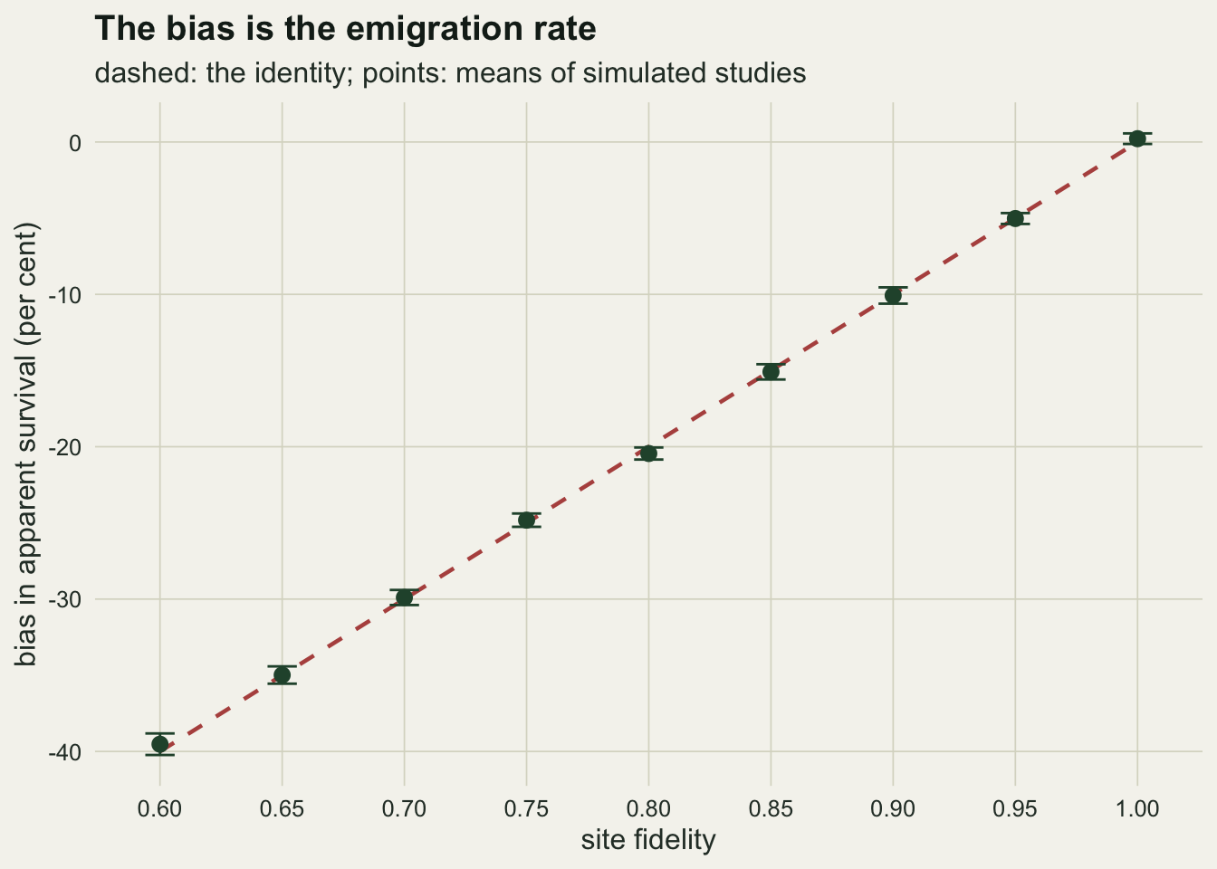
The line holds because every study on that sweep obeys the two conditions. Break each one in turn, with fidelity held to a single value in the fit either way.
n_cond <- 10
cjs_mean <- function(...) {
  est_c <- numeric(n_cond)
  for (b in seq_len(n_cond)) {
    set.seed(3300 + b)
    sim_c <- sim_joint(k_occ, n_cohort, surv = surv_true, plive = plive_true,
                       prec = prec_true, ...)
    est_c[b] <- cjs_fit((sim_c$enc == 1L) * 1L)$est[1]
  }
  mean(est_c)
}
fid_natal <- 0.50; fid_adult <- 0.95; p_away_true <- 0.10
cjs_natal  <- cjs_mean(fid = fid_adult, fid_first = fid_natal)
cjs_seen   <- cjs_mean(fid = fid_true, p_away = p_away_true)
bias_natal <- cjs_natal / surv_true - 1
bias_adult <- -(1 - fid_adult)
bias_seen  <- cjs_seen / surv_true - 1
Ring birds in the nest, let them disperse at 0.50 in their first interval and settle to an adult fidelity of 0.95 afterwards, and the constant-parameter estimate averages 0.669 over 10 studies: 21.3 per cent below true survival, where the adult fidelity on its own would predict 5.0 per cent. One number is being reported for a rate that is not one number, and what comes back is a blend that belongs to no interval of the study. Let emigrants be caught elsewhere with probability 0.10 instead, and the estimate rises to 0.769, 9.5 per cent low rather than 20. With emigrant detection above zero the identity gives the largest shortfall the emigration rate can produce, not the one the study has.
What the separation costs
Returned rings are what buys the split, so the question worth asking is how many of them are needed. Hold the design fixed and vary the reporting probability from a poor scheme to a good one.
rec_grid <- c(0.02, 0.05, 0.10, 0.20, 0.40)
n_cost   <- 20
cost_out <- data.frame(reporting = rec_grid, rings = NA_real_, surv = NA_real_,
                       width_surv = NA_real_, width_fid = NA_real_, n_wide = NA_integer_)
for (i in seq_along(rec_grid)) {
  out_i <- matrix(NA_real_, n_cost, 4)
  for (b in seq_len(n_cost)) {
    set.seed(7000 + 100 * i + b)
    sim_i <- sim_joint(k_occ, n_cohort, surv_true, fid_true, plive_true, rec_grid[i])
    fit_i <- joint_fit(sim_i$enc, sim_i$rel)
    out_i[b, ] <- c(sum(sim_i$enc == 2L), fit_i$est[1],
                    fit_i$hi[1] - fit_i$lo[1], fit_i$hi[2] - fit_i$lo[2])
  }
  cost_out[i, 2:5] <- apply(out_i, 2, median)   # medians: one flat fit must not set the level
  cost_out$n_wide[i] <- sum(out_i[, 4] > 0.99)  # fits that return the whole unit interval
}
cost_out$scaled <- cost_out$width_fid * sqrt(cost_out$rings)
scale_spread <- max(cost_out$scaled) / min(cost_out$scaled) - 1
ring_span   <- max(cost_out$rings) / min(cost_out$rings)
round(cost_out, 3)
reporting rings surv width_surv width_fid n_wide scaled
1 0.02 19.0 0.851 0.370 0.364 1 1.585
2 0.05 48.0 0.847 0.237 0.221 0 1.534
3 0.10 95.0 0.837 0.163 0.156 0 1.518
4 0.20 188.5 0.851 0.116 0.113 0 1.555
5 0.40 372.5 0.856 0.080 0.083 0 1.608At a reporting probability of 0.05 the study gets about 48 rings back and the median fidelity interval is 0.22 wide. That is wide, and it is still an answer: it excludes perfect fidelity, which is the assumption under which the live-only estimate would have been survival. Even at a reporting probability of 0.02, with roughly 19 rings, the median interval is 0.36 wide, although 1 of those 20 fits did come back with the whole unit interval, which is why the table reports medians.
The scaling is the practical part. Multiplying each median interval width by the square root of the median number of recoveries gives 1.58, 1.53, 1.52, 1.56, 1.61 across the five settings: a spread of 6 per cent while the number of returned rings changes by a factor of 20. Precision on the separation is governed by the number of rings that come back, in the ordinary square root way, and that count is the reporting probability multiplied by the number of birds that die under observation.
cost_long <- data.frame(rings = rep(cost_out$rings, 2),
                        width = c(cost_out$width_surv, cost_out$width_fid),
                        target = rep(c("true survival", "site fidelity"), each = nrow(cost_out)))
ref_line <- data.frame(rings = cost_out$rings,
                       width = mean(cost_out$scaled) / sqrt(cost_out$rings))

ggplot(cost_long, aes(rings, width, colour = target)) +
  geom_line(data = ref_line, aes(rings, width), inherit.aes = FALSE,
            colour = te_rust, linetype = "dashed", linewidth = 0.7) +
  geom_line(linewidth = 0.9) + geom_point(size = 2.6) +
  scale_colour_manual(values = c(te_gold, te_forest), name = NULL) +
  scale_x_log10(breaks = round(cost_out$rings)) + scale_y_log10() +
  labs(x = "rings returned per study (log scale)", y = "median interval width (log scale)",
       title = "What a returned ring is worth",
       subtitle = "dashed: proportional to one over the square root of the recovery count") +
  theme_datasheet() + theme(legend.position = "bottom")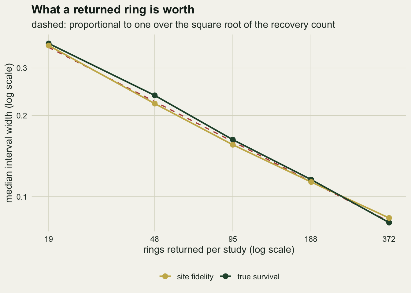
Where the joint model itself breaks
Site fidelity is not the only quantity that multiplies into apparent survival. A ring that falls off does what a bird that leaves does: the animal is alive and on the study area, and it is never recaptured again. Simulate perfect fidelity with an imperfect per interval ring retention instead, and the live-only model returns the same product wearing different clothes.
retain_true <- 0.80
set.seed(5501)
sim_tag   <- sim_joint(k_occ, n_cohort, surv_true, 1, plive_true, prec_true, retain = retain_true)
cj_tag    <- cjs_fit((sim_tag$enc == 1L) * 1L)
jt_tag    <- joint_fit(sim_tag$enc, sim_tag$rel)
tag_pred  <- surv_true * retain_true                          # pseudo-true survival
ps_prec   <- (1 - surv_true) * prec_true / (1 - tag_pred)     # pseudo-true reporting rate
tag_death <- (1 - jt_tag$est[1]) / (1 - surv_true)            # inferred deaths per true death
With a retention rate of 0.80, apparent survival is 0.670 against a predicted product of 0.680: the identity holds with retention substituted for fidelity, which is the bias Arnason and Mills (1981) set out for the Jolly-Seber estimators.
The joint model does not repair it, and where it lands can be written down in advance. From the state alive, on site and still ringed, there are three ways out of an interval: stay, with probability survival times retention; die and become reportable, with probability one minus survival; or shed the ring and leave both channels at once, with probability survival times one minus retention. That is the four-state model of this post at a fidelity of one, so equating the recovery branch of the two processes gives a pseudo-true survival of surv * retain, which is 0.680, and a pseudo-true reporting rate of (1 - surv) * prec / (1 - surv * retain), which is 0.0938. The remaining branches then agree with no further work, and that is checkable by enumeration over every observable history, recoveries included this time.
tr_shed <- matrix(c(tag_pred, 1 - surv_true, surv_true * (1 - retain_true),   # ringed on site
                    0, 0, 1,                                                  # newly dead
                    0, 0, 1), 3, 3, byrow = TRUE)                             # gone for good
em_shed <- rbind(c(1 - plive_true, 1 - prec_true, 1), c(plive_true, 0, 0), c(0, prec_true, 0))
em_ps   <- rbind(c(1 - plive_true, 1, 1 - ps_prec, 1), c(plive_true, 0, 0, 0), c(0, 0, ps_prec, 0))
obs_all <- as.matrix(expand.grid(rep(list(0:2), k_occ - 1)))
p_shed  <- apply(obs_all, 1, fwd_obs, tr = tr_shed, em = em_shed)
p_ps    <- apply(obs_all, 1, fwd_obs, tr = mat_four(tag_pred, 1), em = em_ps)
stopifnot(isTRUE(all.equal(sum(p_shed), 1)), isTRUE(all.equal(sum(p_ps), 1)))
n_obs <- nrow(obs_all); shed_gap <- max(abs(p_shed - p_ps))
Over all 2187 observable histories the ring loss process and the joint model at those pseudo-true values give probabilities that are equal to within floating-point rounding. Ring loss is not an approximation to the joint model: it is the joint model, at another point in the same parameter space. Nothing is left over to test, so neither model can be told that anything is wrong, and a goodness of fit check has no lack of fit to find.
The fit goes to that neighbourhood. Survival comes back at 0.669, next to the pseudo-true 0.680, and the reporting probability at 0.073 against a true 0.20. The model absorbs the shed rings by concluding that many more birds died and far fewer of the dead were found: the inferred death rate is 2.2 times the true one, and the rings that fail to come back are then explained by a reporting rate just over a third of the truth. Ring loss cannot be booked as emigration, because an emigrant keeps its ring and can still be reported dead, while a shed ring leaves both channels at once. The fidelity of one is the exact pseudo-true value, not a lucky landing.
n_tag   <- 40
tag_out <- matrix(NA_real_, n_tag, 3)
for (b in seq_len(n_tag)) {
  set.seed(5500 + b)
  sim_t <- sim_joint(k_occ, n_cohort, surv_true, 1, plive_true, prec_true, retain = retain_true)
  fit_t <- joint_fit(sim_t$enc, sim_t$rel)
  tag_out[b, ] <- c(fit_t$est[1], fit_t$est[4], fit_t$par[2])
}
tag_med  <- apply(tag_out[, 1:2], 2, median); tag_over <- sum(tag_out[, 1] > surv_true)
tag_bound <- sum(tag_out[, 3] > 6)        # a fidelity logit above 6 is the boundary
That study is one draw and a low one on reporting. Over 40 fresh studies at the same settings the median survival estimate is 0.685 and the median reporting estimate 0.0951, against pseudo-true values of 0.680 and 0.0938, and 0 of the 40 put survival above the true 0.85. The estimator is not noisy about survival here, it is pointed somewhere else.
Fidelity needs separate care in the reporting, because in 23 of those 40 studies, the worked one included, it is a boundary maximum rather than an estimate.
fid_logit <- jt_tag$par[2]
eig_tag   <- min(eigen(jt_tag$hess, only.values = TRUE)$values)
prof_dev  <- function(fv) {
  nll_f <- function(p) joint_nll(c(p[1], qlogis(fv), p[2], p[3]), sim_tag$enc, sim_tag$rel)
  2 * (optim(qlogis(c(0.7, 0.4, 0.15)), nll_f, method = "BFGS",
             control = list(maxit = 2000, reltol = 1e-12))$value - jt_tag$nll)
}
fid_axis <- seq(0.86, 0.999, length.out = 12)
prof_out <- data.frame(fid = fid_axis, dev = vapply(fid_axis, prof_dev, numeric(1)))
crit_1   <- qchisq(0.95, 1)
fid_prof <- approx(prof_out$dev, prof_out$fid, xout = crit_1)$y
The fitted fidelity is 1.0000, which is a logit of 12.1; the smallest eigenvalue of the Hessian is \(4.2 \times 10^{-5}\), and the Wald interval the fitting function returns from it is 0.000 to 1.000, the whole unit interval. A Wald interval at a boundary is not an interval, it is an artefact of a flat curvature, and quoting the point estimate alone hides that. The profile likelihood is the thing to report: the deviance from holding fidelity away from its maximum crosses 3.84 at 0.93, so the 95 per cent set runs from there to one.
ggplot(prof_out, aes(fid, dev)) +
  geom_hline(yintercept = crit_1, linetype = "dashed", colour = te_rust, linewidth = 0.7) +
  geom_segment(x = fid_prof, xend = fid_prof, y = 0, yend = crit_1,
               colour = te_gold, linewidth = 0.7) +
  geom_line(colour = te_forest, linewidth = 0.9) +
  geom_point(colour = te_forest, size = 2) +
  labs(x = "site fidelity", y = "profile deviance",
       title = "The fidelity maximum is on the boundary",
       subtitle = "dashed: the 95 per cent cutoff; gold: the lower end of the profile set") +
  theme_datasheet()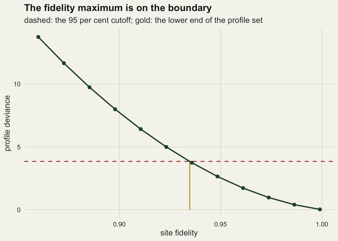
Ring loss is one assumption failing. The transition matrix carries another that is easier to miss: the row for emigrants uses the same survival as the row for residents, so a bird that leaves is assumed to die at the residents’ rate for the rest of the study. No recapture and no recovery in this design speaks to it directly. Refit the same model to studies where it is false.
emi_set <- c(surv_true, 0.95, 0.60)
n_emi   <- 30
emi_run <- function(sa) {
  o_e <- matrix(NA_real_, n_emi, 4)
  for (b in seq_len(n_emi)) {
    set.seed(4400 + b)
    s_e <- sim_joint(k_occ, n_cohort, surv_true, fid_true, plive_true, prec_true, surv_away = sa)
    f_e <- joint_fit(s_e$enc, s_e$rel)
    o_e[b, ] <- c(f_e$lo[1] < surv_true && f_e$hi[1] > surv_true, f_e$est[1], f_e$est[4],
                  cjs_fit((s_e$enc == 1L) * 1L)$est[1])
  }
  c(colMeans(o_e), sd(o_e[, 4]) / sqrt(n_emi))
}
emi_out <- as.data.frame(cbind(surv_away = emi_set, t(sapply(emi_set, emi_run))))
names(emi_out)[2:6] <- c("covered", "survival", "reporting", "cjs", "cjs_se")
emi_out$covered <- emi_out$covered * n_emi
report_off <- emi_out$reporting[2] / prec_true - 1
round(emi_out, 4)
surv_away covered survival reporting cjs cjs_se
1 0.85 30 0.8478 0.2012 0.6799 0.0014
2 0.95 2 0.7603 0.1268 0.6836 0.0021
3 0.60 30 0.8921 0.3275 0.6813 0.0022With emigrants dying at the residents’ rate the survival interval covers the truth in 30 of 30 studies. Let emigrants survive at 0.95 instead of 0.85 and coverage falls to 2 of 30, with the reporting probability 37 per cent low. Let them survive at 0.60 and the damage lands the other way, on the reporting rate rather than on coverage. The live-only estimate stays where it was: the three batches average 0.6799, 0.6836 and 0.6813, spread no wider than a few Monte Carlo standard errors of 0.0022, and it cannot move in principle, because a bird that has left contributes nothing to the recapture column whatever it does next. The identity survives this assumption and the joint model does not, which is part of the price of asking the data a harder question.
set.seed(4401)
sim_bad <- sim_joint(k_occ, n_cohort, surv_true, fid_true, plive_true, prec_true,
                     surv_away = emi_set[2])
ctl_5 <- list(maxit = 4000, reltol = 1e-12)
opt_4p <- optim(qlogis(c(0.7, 0.7, 0.4, 0.15)), joint_nll, enc = sim_bad$enc, rel = sim_bad$rel,
                method = "BFGS", control = ctl_5)
opt_5p <- optim(qlogis(c(0.7, 0.7, 0.4, 0.15, 0.7)), joint_nll, enc = sim_bad$enc,
                rel = sim_bad$rel, method = "BFGS", hessian = TRUE, control = ctl_5)
dev_emi <- 2 * (opt_4p$value - opt_5p$value); eig_5p <- min(eigen(opt_5p$hessian)$values)
The obvious repair is to give emigrants their own survival, and on data of this shape it does not work. Fitted to the misspecified study, the five-parameter version gains a deviance of 2.48 against a cutoff of 3.84, so the test says nothing is wrong; the smallest eigenvalue of its Hessian is \(1.2 \times 10^{-5}\), so the extra parameter is not being estimated so much as pushed to a boundary. The assumption has to be argued from natural history, not from the likelihood.
What to report
Give the two encounter columns separately: birds marked per occasion, live recaptures per occasion, rings returned per occasion. The last of those is the sample size for everything the joint model adds, and a reader cannot judge a fidelity estimate without it.
Say which survival is being reported. If the model is live only, the quantity is apparent survival, it estimates the product of survival and site fidelity, and calling it survival is wrong unless the population is closed to permanent emigration. Lebreton and colleagues settled this vocabulary in 1992 and it still slips.
If fidelity is estimated, report it with its interval and with the number of recoveries beside it, because the width tracks the square root of that count. An estimate from a handful of rings is a real estimate with a wide interval, not a decorative one. If the maximum sits on one, say so and give a profile set: a Wald interval computed at a boundary is not an interval.
State the assumed geometry of emigration. The model here treats leaving as permanent and absorbing, and if animals come and go, this is the wrong model and the temporary absence machinery belongs in its place. Report the ring retention assumption in the same breath, or measure it by double marking: both models here assume marks are permanent, and neither can detect that they are not.
Honest limits
Survival and the reporting probability are estimated from the same returned rings, and they move together rather than trading off. Across the 200 replicate studies their correlation is 0.88: the studies in the lowest quarter of the reporting estimate average 0.819 for survival, those in the highest quarter 0.883. A fixed haul of returned rings is roughly the death rate multiplied by the reporting rate, so the two stories one study cannot separate are many died and few were found against few died and most were found. The same ridge is inside a single fit: in the worked study the Hessian puts survival against reporting at 0.89. The correlation that costs more is a different one, survival against fidelity at -0.91 in that study and -0.92 across the replicates. Holding the reporting probability at its true value narrows the survival interval of the worked study from 0.1111 to 0.0524; holding fidelity narrows it to 0.0463.
Everything above holds survival, fidelity, recapture and reporting constant across occasions and across individuals. Real reporting probabilities are not: they drift as public reporting habits change, they differ between hunted and unhunted species, and they depend on where a bird dies. Barker (1999) treats the age dependent and marking effect versions, and Kendall and colleagues (2013) fold recoveries into a design that also carries auxiliary resightings. Emigration here is permanent and unobserved, while a real study sits somewhere between that and the temporary absence of the neighbouring post.
The recovery process is assumed to be indifferent to state: an emigrant that dies is as likely to be reported as a resident that dies. Birds that leave a colony often leave the region where rings are looked for at all, and the fidelity estimate quietly absorbs the difference. The emigrant row of the transition matrix makes the same kind of assumption about survival, and the asymmetry measured above is the part to carry away: what emigrants do after they leave cannot touch the live-only identity, while it moves the joint model’s survival estimate off the truth and can take its interval coverage with it. Separating survival from fidelity is bought with assumptions about animals that are never seen again, and the four-state chain has no state for a bird that is alive, on site and no longer carrying a ring, which is why double marking rather than a longer likelihood is the answer to ring loss.
References
Seber GAF 1970 Biometrika 57(2):313-318 (10.1093/biomet/57.2.313)
Arnason AN, Mills KH 1981 Canadian Journal of Fisheries and Aquatic Sciences 38(9):1077-1095 (10.1139/f81-148)
Lebreton JD, Burnham KP, Clobert J, Anderson DR 1992 Ecological Monographs 62(1):67-118 (10.2307/2937171)
Barker RJ 1997 Biometrics 53(2):666-677 (10.2307/2533966)
Barker RJ 1999 Bird Study 46(sup1):S82-S91 (10.1080/00063659909477235)
Lebreton JD, Almeras T, Pradel R 1999 Bird Study 46(sup1):S39-S46 (10.1080/00063659909477230)
Gilroy JJ, Virzi T, Boulton RL, Lockwood JL 2012 Ecology 93(7):1509-1516 (10.1890/12-0124.1)
Kendall WL, Barker RJ, White GC, Lindberg MS, Langtimm CA, Penaloza CL 2013 Methods in Ecology and Evolution 4(9):828-835 (10.1111/2041-210X.12077)