library(ggplot2)

te_ink <- "#16241d"; te_forest <- "#275139"; te_gold <- "#c9b458"
te_rust <- "#b5534e"; te_sage <- "#93a87f"; te_line <- "#dad9ca"; te_muted <- "#5d6b61"

theme_te <- function() {
  theme_minimal(base_size = 12) +
    theme(
          plot.background  = element_rect(fill = "#f5f4ee", colour = NA),
          panel.background = element_rect(fill = "#f5f4ee", colour = NA),
          text = element_text(colour = te_ink),
          plot.title = element_text(face = "bold", colour = te_ink),
          plot.subtitle = element_text(colour = te_muted, size = rel(0.9)),
          axis.text = element_text(colour = te_muted),
          panel.grid.major = element_line(colour = te_line, linewidth = 0.3),
          panel.grid.minor = element_blank(),
          legend.position = "top", legend.title = element_blank())
}Checking an open-population model
R
capture-recapture
model diagnostics
population ecology
ecology tutorial
Capture-recapture goodness-of-fit tests take first capture as given. Work out what that leaves out, and why a clean test is no licence to believe the abundance.
Corrected 7 October 2026: the post said that the goodness-of-fit tests people actually run are parametric bootstraps; it now says that they work on finite data and calls the parametric bootstrap one of them.
Corrected 30 September 2026: the post said that every standard goodness-of-fit test is computed on the m-array; it now says that they all take the first capture as given, with the m-array as the simplest such summary. The closing section paired growth-rate and abundance errors from two different simulated worlds as if they were general; it now ties each to the world it came from.
Three posts in, the pattern is hard to miss. Change the first-capture probability and survival does not move, the growth rate moves a little, and in the first post’s trap-response world the superpopulation loses 39 per cent of the animals. Every practitioner’s next question is the right one: would a goodness-of-fit test have told me?
This post answers it exactly, and the answer is not “the test has low power”. It is worse and more interesting than that.
What a goodness-of-fit test looks at
Every standard capture-recapture goodness-of-fit test (the Test 2 and Test 3 components in RELEASE and U-CARE, and the parametric bootstrap in MARK) is computed on what happens to animals after their first capture, taking that capture as given. The simplest summary of that information is the m-array, and it is the one this post works with. Take every animal, every time it is captured, and ask when it was next seen. Row t holds the R_t animals released at t; cell (t, j) counts how many of them were next caught at j.
marray <- function(H) {
  k <- ncol(H); m <- matrix(0, k - 1, k); R <- numeric(k - 1)
  for (i in seq_len(nrow(H))) {
    w <- which(H[i, ] == 1)
    for (a in seq_along(w)) {
      t <- w[a]; if (t == k) next
      R[t] <- R[t] + 1
      if (a < length(w)) m[t, w[a + 1]] <- m[t, w[a + 1]] + 1
    }
  }
  list(R = R, m = m[, -1, drop = FALSE])
}
ma_prob <- function(phi, p, k) {
  P <- matrix(0, k - 1, k - 1)
  for (t in 1:(k - 1)) for (j in t:(k - 1)) {
    q <- phi^(j - t + 1) * p
    if (j > t) q <- q * prod(rep(1 - p, j - t))
    P[t, j] <- q
  }
  P
}
ma_exp <- function(R, phi, p) sweep(ma_prob(phi, p, length(R) + 1), 1, R, "*")
gof_chi2 <- function(R, m, phi, p) {
  E <- ma_exp(R, phi, p)
  O <- cbind(m, R - rowSums(m)); Ex <- cbind(E, R - rowSums(E))
  keep <- Ex > 1e-9
  sum((O[keep] - Ex[keep])^2 / Ex[keep])
}
Read the first line of marray again. An animal enters the table when it is released, which means when it has already been caught. The releases R_t are the row totals, taken as given. Nothing in this table is a statement about how an animal came to be marked in the first place.
That is not an oversight. It is the same conditioning that makes the Cormack-Jolly-Seber model safe, and the goodness-of-fit test is a test of that model, so it inherits exactly the same blind spot. The question is how big the blind spot is, and the answer is available in closed form.
The claim, stated so that it can fail
Here is the claim. In a trap-response world (naive animals caught with probability pf, marked animals with pr), the process generating the marked animals’ futures is Cormack-Jolly-Seber with parameters phi and pr. Not approximately: exactly. The first-capture probability pf decides which animals get into the m-array, and nothing else. It appears in no cell.
If that is right, the expected m-array in the trap-response world is the expected m-array under CJS(phi, pr), the test statistic has no non-centrality, and the test has no power against this violation. Not low power. None.
A claim like that is easy to “verify” in a way that cannot fail: compute the CJS expectation, compare it with the CJS expectation, and announce that the difference is zero. So do it the other way. Enumerate all 64 capture histories, weight each by its exact probability under the world’s own law, build the m-array those weights imply, and compare it with the m-array expected at the best-fitting CJS. That comparison can fail, and one of the three worlds below fails it.
sim_js <- function(N, beta, phi, p, seed, pf = p) {
  set.seed(seed); k <- length(beta)
  e <- sample.int(k, N, replace = TRUE, prob = beta)
  Alive <- matrix(FALSE, N, k)
  Alive[cbind(seq_len(N), e)] <- TRUE
  for (t in 2:k) Alive[, t] <- Alive[, t] | (Alive[, t - 1] & runif(N) < phi)
  H <- matrix(0L, N, k); seen <- rep(FALSE, N)
  for (t in seq_len(k)) {
    H[, t] <- as.integer(Alive[, t] & runif(N) < ifelse(seen, p, pf))
    seen <- seen | H[, t] == 1L
  }
  list(H = H, Alive = Alive)
}
## trap DEPENDENCE: the recapture probability depends on capture at t-1
sim_td <- function(N, beta, phi, pA, pB, seed) {
  set.seed(seed); k <- length(beta)
  e <- sample.int(k, N, replace = TRUE, prob = beta)
  Al <- matrix(FALSE, N, k); Al[cbind(seq_len(N), e)] <- TRUE
  for (t in 2:k) Al[, t] <- Al[, t] | (Al[, t - 1] & runif(N) < phi)
  H <- matrix(0L, N, k); prev <- rep(FALSE, N)
  for (t in seq_len(k)) {
    H[, t] <- as.integer(Al[, t] & runif(N) < ifelse(prev, pA, pB))
    prev <- H[, t] == 1L
  }
  list(H = H, Alive = Al)
}
hsum <- function(H) {
  k <- ncol(H); idx <- col(H) * H; idx[idx == 0] <- NA
  list(f = suppressWarnings(apply(idx, 1, min, na.rm = TRUE)),
       l = suppressWarnings(apply(idx, 1, max, na.rm = TRUE)),
       s = rowSums(H), k = k)
}
chi_vec <- function(phi, p, k) {
  chi <- numeric(k); chi[k] <- 1
  for (j in (k - 1):1) chi[j] <- (1 - phi) + phi * (1 - p) * chi[j + 1]
  chi
}
cjs_nll <- function(par, S, fr = 1) {
  phi <- plogis(par[1]); p <- plogis(par[2]); chi <- chi_vec(phi, p, S$k)
  v <- -sum(fr * log(phi^(S$l - S$f) * p^(S$s - 1) * (1 - p)^(S$l - S$f - S$s + 1) * chi[S$l]))
  if (!is.finite(v)) 1e10 else v
}
## the everyday fit: one dataset, optim's default stopping rule
fit_cjs <- function(H) {
  S <- hsum(H[rowSums(H) > 0, , drop = FALSE])
  o <- optim(c(qlogis(0.7), qlogis(0.3)), cjs_nll, S = S, method = "BFGS")
  list(phi = plogis(o$par[1]), p = plogis(o$par[2]))
}
## the probability-limit fit: expected frequencies, tolerance tightened on purpose
fit_cjs_f <- function(A, fr) {
  ok <- rowSums(A) > 0; S <- hsum(A[ok, , drop = FALSE])
  o <- optim(c(qlogis(0.7), qlogis(0.3)), cjs_nll, S = S, fr = fr[ok], method = "BFGS",
             control = list(reltol = 1e-14, maxit = 5000))
  list(phi = plogis(o$par[1]), p = plogis(o$par[2]))
}
all_hist <- function(k) as.matrix(expand.grid(rep(list(0:1), k))[, k:1])
Two fitters, and the difference between them is the point of the section. When you fit one dataset, optim’s default stopping rule is far finer than the sampling noise, so it does not matter. When you are measuring whether a deviation is zero, the optimiser’s own error is the entire error budget: at the default tolerance the model-true world reports a small non-zero non-centrality, which is the stopping rule being measured, not the model.
popan_ph2 <- function(S, phi, pf, p, beta) {
k <- S$k; chi <- chi_vec(phi, p, k)
nu <- numeric(k); nu[k] <- 1 - pf
for (e in (k - 1):1) nu[e] <- (1 - pf) * ((1 - phi) + phi * nu[e + 1])
x <- phi * (1 - pf); g <- numeric(k); g[1] <- beta[1]
for (f in 2:k) g[f] <- x * g[f - 1] + beta[f]
out <- numeric(length(S$s)); out[S$s == 0] <- sum(beta * nu)
ok <- S$s > 0; f <- S$f[ok]; l <- S$l[ok]; s <- S$s[ok]
out[ok] <- g[f] * pf * phi^(l - f) * p^(s - 1) * (1 - p)^(l - f - s + 1) * chi[l]
out
}
## exact history probability under trap dependence: three-state forward pass
ph_td <- function(A, phi, pA, pB, beta) {
k <- ncol(A); out <- numeric(nrow(A))
for (i in seq_len(nrow(A))) {
h <- A[i, ]; tot <- 0
for (e in seq_len(k)) { # entry occasion
if (e > 1 && any(h[1:(e - 1)] == 1L)) next
al <- c(1, 0, 0); ok <- TRUE # alive¬-caught-last, alive&caught-last, dead
for (t in e:k) {
if (t > e) {
nx <- c(0, 0, 0); nx[h[t - 1] + 1] <- phi * (al[1] + al[2])
nx[3] <- (1 - phi) * (al[1] + al[2]) + al[3]; al <- nx
}
al <- al * (if (h[t] == 1L) c(pB, pA, 0) else c(1 - pB, 1 - pA, 1))
if (sum(al) == 0) { ok <- FALSE; break }
}
if (ok) tot <- tot + beta[e] * sum(al)
}
out[i] <- tot
}
out
}
## m-array expectation implied by a law over histories
ma_expect <- function(A, ph) {
k <- ncol(A); R <- numeric(k - 1); m <- matrix(0, k - 1, k - 1)
for (i in seq_len(nrow(A))) {
w <- which(A[i, ] == 1L)
for (a in seq_along(w)) {
t <- w[a]; if (t == k) next
R[t] <- R[t] + ph[i]
if (a < length(w)) m[t, w[a + 1] - 1] <- m[t, w[a + 1] - 1] + ph[i]
}
}
list(R = R, m = m)
}
nc_marray <- function(A, ph, scale) {
S <- hsum(A)
f <- fit_cjs_f(A, scale * ph)
e <- ma_expect(A, scale * ph)
Ecjs <- ma_exp(e$R, f$phi, f$p)
O <- cbind(e$m, e$R - rowSums(e$m)); E <- cbind(Ecjs, e$R - rowSums(Ecjs))
keep <- E > 1e-9
list(phi = f$phi, p = f$p, rel = max(abs(e$m - Ecjs)) / max(e$m),
nc = sum((O[keep] - E[keep])^2 / E[keep]), ncell = sum(keep))
}
k <- 6; phi <- 0.80; Nsup <- 400
beta <- c(0.42, 0.14, 0.12, 0.12, 0.10, 0.10)
pf <- 0.20; pr <- 0.45
A <- all_hist(k); S <- hsum(A)
worlds <- list("model-true" = popan_ph2(S, phi, 0.35, 0.35, beta),
"trap response" = popan_ph2(S, phi, pf, pr, beta),
"trap dependence" = ph_td(A, phi, pA = 0.60, pB = 0.22, beta))
tab <- t(sapply(worlds, function(pv) {
q <- nc_marray(A, pv, 1e6); s <- nc_marray(A, pv, Nsup)
df <- q$ncell - (k - 1) - 2
c(mass = sum(pv), phi = q$phi, p = q$p, rel_dev = q$rel, nc = s$nc, df = df,
power = pchisq(qchisq(0.95, df), df, ncp = s$nc, lower.tail = FALSE))
}))
round(tab[, c("mass", "phi", "p", "rel_dev", "nc", "power")], 6) mass phi p rel_dev nc power
model-true 1 0.800000 0.350000 0.00000 0.00000 0.050000
trap response 1 0.800000 0.450000 0.00000 0.00000 0.050000
trap dependence 1 0.681217 0.671503 0.09471 15.95384 0.741346Each of the three laws sums to one, so each is a probability distribution over the 64 histories and the enumeration is right.
In the model-true world the best-fitting CJS is (0.8000, 0.3500) and the largest m-array cell deviates by \(4.2 \times 10^{-8}\) of the largest cell. Nothing to see: the model is true.
In the trap-response world the best-fitting CJS is (0.8000, 0.4500). Look at those two numbers. The survival is the true survival, and the capture probability is exactly pr, the recapture probability, 0.45. The largest cell deviates by \(2.9 \times 10^{-8}\). The non-centrality at study size is 0.000, and the implied power of a 5 per cent test is 0.050, which is the size of the test. A test with power equal to its size is a coin.
In the trap-dependence world, where the recapture probability depends on whether the animal was caught at t - 1 (0.60 if it was, 0.22 if it was not), the same machinery gives a largest deviation of 9.47 per cent, a non-centrality of 15.95 on 13 degrees of freedom, and implied power 0.741.
So the check is a real check. It fails when it should.
The distinction that decides everything
Both of those worlds are “trap-happy animals”. They are not the same thing, and the m-array can see exactly one of them.
Trap response is a change at the moment of marking: naive animals are caught with one probability, marked animals with another. Once an animal is in the m-array, it behaves like every other animal in the m-array, forever. The heterogeneity lives entirely on the boundary the m-array conditions across.
Trap dependence is a change within the marked animals: caught last time makes you easier (or harder) to catch this time. That is a statement about the gaps between recaptures, and gaps between recaptures are precisely what the m-array is made of.
The test is not weak. It is aimed somewhere else.
Does the real machinery agree?
That was arithmetic on expected values. The tests people actually run work on finite data, and one of them is a parametric bootstrap with an estimated null and a c-hat. Run one properly: fit CJS, compute the m-array chi-square, simulate B datasets from the fitted model holding the observed first-capture times fixed, and compare.
sim_cjs_hist <- function(ft, k, phi, p, seed) {
  set.seed(seed); n <- length(ft)
  H <- matrix(0L, n, k); H[cbind(seq_len(n), ft)] <- 1L
  alive <- rep(TRUE, n)
  for (t in 2:k) {
    up <- ft < t
    if (!any(up)) next
    alive[up] <- alive[up] & (runif(sum(up)) < phi)
    d <- up & alive & (runif(n) < p)
    H[d, t] <- 1L
  }
  H
}
gof_boot <- function(H, B, seed) {
  k <- ncol(H); a <- marray(H); f <- fit_cjs(H)
  obs <- gof_chi2(a$R, a$m, f$phi, f$p)
  ft <- max.col(H > 0, ties.method = "first")
  nl <- numeric(B)
  for (j in 1:B) {
    Hs <- sim_cjs_hist(ft, k, f$phi, f$p, seed + j)
    Hs <- Hs[rowSums(Hs) > 0, , drop = FALSE]
    as <- marray(Hs); fs <- tryCatch(fit_cjs(Hs), error = function(e) f)
    nl[j] <- gof_chi2(as$R, as$m, fs$phi, fs$p)
  }
  list(p = mean(nl >= obs), chat = obs / mean(nl))
}
The abundance estimate comes from the POPAN model of the first post, unchanged. It is here so that every simulated study reports a goodness-of-fit verdict and a superpopulation estimate side by side.
nu_vec <- function(phi, p, k) {
  nu <- numeric(k); nu[k] <- 1 - p
  for (e in (k - 1):1) nu[e] <- (1 - p) * ((1 - phi) + phi * nu[e + 1])
  nu
}
ent_vec <- function(phi, p, beta, k) {
  x <- phi * (1 - p); g <- numeric(k); g[1] <- beta[1]
  for (f in 2:k) g[f] <- x * g[f - 1] + beta[f]
  g
}
popan_ph <- function(S, phi, p, beta) {
  k <- S$k; chi <- chi_vec(phi, p, k); g <- ent_vec(phi, p, beta, k)
  ok <- S$s > 0; out <- numeric(length(S$s))
  out[!ok] <- sum(beta * nu_vec(phi, p, k))
  f <- S$f[ok]; l <- S$l[ok]; s <- S$s[ok]
  out[ok] <- g[f] * p * phi^(l - f) * p^(s - 1) * (1 - p)^(l - f - s + 1) * chi[l]
  out
}
popan_nll <- function(par, freq, S, n) {
  k <- S$k
  N <- n + exp(par[1]); phi <- plogis(par[2]); p <- plogis(par[3])
  bl <- c(0, par[4:(k + 2)]); beta <- exp(bl) / sum(exp(bl))
  ph <- popan_ph(S, phi, p, beta)
  P0 <- ph[S$s == 0]
  if (!is.finite(P0) || P0 <= 0 || P0 >= 1) return(1e10)
  pv <- ph[S$s > 0]; if (any(!is.finite(pv)) || any(pv <= 0)) return(1e10)
  v <- -(lgamma(N + 1) - lgamma(N - n + 1) + (N - n) * log(P0) + sum(freq * log(pv)))
  if (!is.finite(v)) 1e10 else v
}
fit_popan_N <- function(H, k) {
  SA <- hsum(A); keyA <- apply(A, 1, paste, collapse = "")
  seen <- apply(H[rowSums(H) > 0, , drop = FALSE], 1, paste, collapse = "")
  n <- length(seen)
  freq <- as.integer(table(factor(seen, levels = keyA[SA$s > 0])))
  o <- optim(c(log(0.5 * n), qlogis(0.7), qlogis(0.3), rep(0, k - 1)), popan_nll,
             freq = freq, S = SA, n = n, method = "BFGS",
             control = list(maxit = 5000, reltol = 1e-13))
  n + exp(o$par[1])
}
M <- 200; B <- 40
go <- function(gen) {
P <- CH <- NN <- numeric(M)
for (b in 1:M) {
d <- gen(b); H <- d$H[rowSums(d$H) > 0, , drop = FALSE]
g <- gof_boot(H, B, seed = 500000 + b * 1000)
P[b] <- g$p; CH[b] <- g$chat
NN[b] <- tryCatch(fit_popan_N(d$H, k), error = function(e) NA)
}
data.frame(p = P, chat = CH, N = NN)
}
res <- suppressWarnings(list(
`model-true` = go(function(b) sim_js(Nsup, beta, phi, 0.35, seed = 60000 + b)),
`trap response` = go(function(b) sim_js(Nsup, beta, phi, pr, seed = 61000 + b, pf = pf)),
`trap dependence` = go(function(b) sim_td(Nsup, beta, phi, pA = 0.60, pB = 0.22,
seed = 62000 + b))))
smry <- t(sapply(res, function(d) c(reject = mean(d$p < 0.05), mean_p = mean(d$p),
chat = mean(d$chat), N = mean(d$N, na.rm = TRUE),
N_err = 100 * (mean(d$N, na.rm = TRUE) / Nsup - 1))))
round(smry, 3) reject mean_p chat N N_err
model-true 0.035 0.491 1.015 397.792 -0.552
trap response 0.030 0.506 0.988 244.186 -38.953
trap dependence 0.715 0.061 3.528 226.650 -43.337The measured rejection rates are 0.035, 0.030 and 0.715, against implied powers of 0.050, 0.050 and 0.741 from the non-centrality. The arithmetic predicted the simulation, including the hard one.
df_p <- data.frame(
  world = factor(rep(rownames(tab), 2), levels = rownames(tab)),
  value = c(tab[, "power"], smry[, "reject"]),
  kind = rep(c("implied by the non-centrality", "measured over 200 studies"), each = 3))
ggplot(df_p, aes(world, value, fill = kind)) +
  geom_col(position = position_dodge(width = 0.7), width = 0.62) +
  geom_hline(yintercept = 0.05, colour = te_ink, linetype = 2, linewidth = 0.6) +
  annotate("text", x = 0.55, y = 0.085, label = "nominal 5 per cent", colour = te_ink,
           hjust = 0, size = 3.4) +
  scale_fill_manual(values = c(`implied by the non-centrality` = te_sage,
                               `measured over 200 studies` = te_forest)) +
  scale_y_continuous(labels = function(x) sprintf("%.0f%%", 100 * x)) +
  labs(title = "The test does exactly what the algebra says",
       subtitle = "Rejection rate of the m-array goodness-of-fit test at the 5 per cent level",
       x = NULL, y = "Rejection rate") +
  theme_te()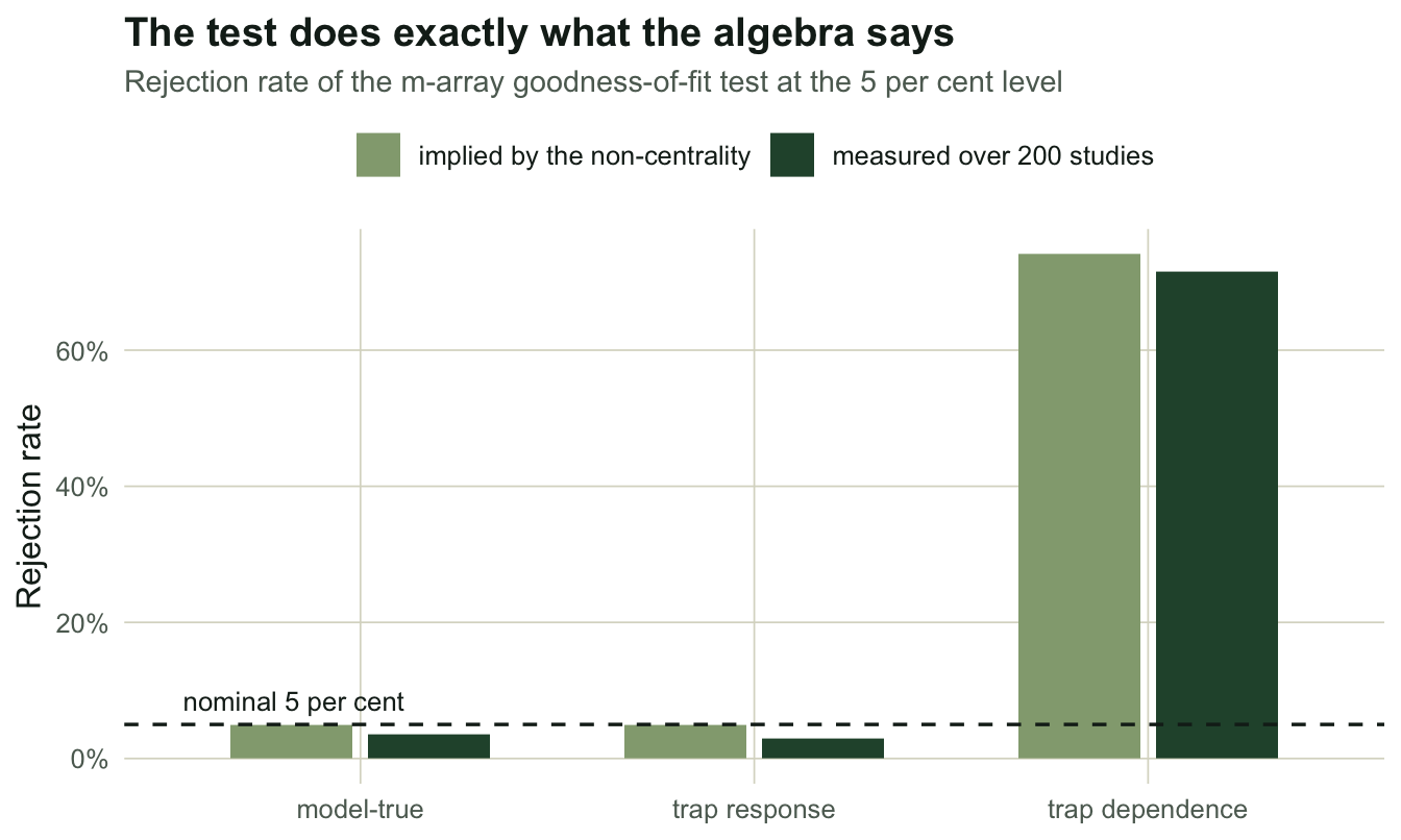
The part worth reading twice
Now put the verdict next to the answer.
df_v <- do.call(rbind, lapply(names(res), function(nm)
  data.frame(world = nm, chat = res[[nm]]$chat, N = res[[nm]]$N)))
df_v$world <- factor(df_v$world, levels = rownames(tab))
ggplot(df_v, aes(chat, N, colour = world)) +
  geom_hline(yintercept = Nsup, colour = te_ink, linetype = 2, linewidth = 0.8) +
  geom_vline(xintercept = 1, colour = te_line, linewidth = 0.6) +
  geom_point(alpha = 0.55, size = 1.9) +
  annotate("text", x = 5.4, y = Nsup + 14, label = "truth", colour = te_ink,
           hjust = 1, size = 3.6, fontface = "bold") +
  scale_colour_manual(values = c(`model-true` = te_forest, `trap response` = te_rust,
                                 `trap dependence` = te_gold)) +
  labs(title = "A clean bill of health is not an accurate answer",
       subtitle = "200 studies per world; c-hat near 1 means the fit is fine",
       x = "c-hat from the parametric bootstrap", y = "Estimated superpopulation") +
  theme_te()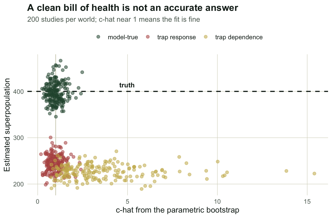
The rust cloud is the whole series in one picture. Those studies have a c-hat of 0.988, an average bootstrap p-value of 0.506, and a rejection rate of 3.0% against a nominal five. By every diagnostic you would report in a paper, the model fits. There is nothing to correct: a c-hat below one does not even license inflating the standard errors. And the superpopulation estimate averages 244.2 against a true 400, an error of -39.0%.
Compare the gold cloud. Trap dependence gets caught 71.5% of the time with a c-hat of 3.528. The machinery works. Given a violation it can see, it sees it.
So what do you do?
The honest answer is that this failure is not fixable by testing harder, because it is not a testing problem. The information required to detect it is not in the data. The m-array cannot tell you about first captures for the same reason the CJS likelihood cannot: they were conditioned away, and that conditioning is why the survival estimate is trustworthy. You cannot keep the protection and also see through it.
What is left is not nothing.
Run the test anyway. It catches trap dependence, transience, and the other violations that live inside the marked animals, and those are common. A c-hat of 3.53 is worth knowing about.
Then treat the result as what it is: evidence about the marked animals, and silence about everyone else. If the study reports survival, that silence costs nothing. If it reports abundance, the number rests on an assumption that no diagnostic in the output speaks to, and it should be argued for in the methods section instead: what is known about the marking process, whether handling changes behaviour in this species, whether the first capture plausibly works like a recapture.
Or change the data. The robust design post is what that looks like: information the likelihood cannot conjure, bought in the field. That has its own honest limits, and they are also not visible in a goodness-of-fit test.
What to take away
A goodness-of-fit test answers one question: is the model consistent with the data it was fitted to? That is not the same question as: is the number I care about correct. Across this series the same structure has appeared four times. Survival is exact because it declines to model first capture. In the trap-response world of the seniority post, the growth rate is 4 per cent off because it half-models it, and abundance is nearly half off because it fully depends on it (39 per cent off in the trap-response world used here). And the test that should adjudicate is computed on an object that conditions first capture away, so it returns a clean verdict in every one of those cases.
The generalisable move is to ask, of any diagnostic, which part of the model does this statistic touch? If your headline number depends on a part the statistic does not touch, a clean test tells you nothing about it. That is not a failure of the test. It is a fact about where the information is, and the only honest response is to say so in the paper.
References
Pollock, Nichols, Brownie & Hines 1990 Wildlife Monographs 107:1-97
Pollock, Hines & Nichols 1985 Biometrics 41:399-410 (10.2307/2530865)
Schwarz & Arnason 1996 Biometrics 52:860-873 (10.2307/2533048)
Link 2003 Biometrics 59(4):1123-1130 (10.1111/j.0006-341X.2003.00129.x)