library(ggplot2)

te_ink <- "#16241d"; te_forest <- "#275139"; te_gold <- "#c9b458"
te_rust <- "#b5534e"; te_sage <- "#93a87f"; te_line <- "#dad9ca"; te_muted <- "#5d6b61"

theme_te <- function() {
  theme_minimal(base_size = 12) +
    theme(
          plot.background  = element_rect(fill = "#f5f4ee", colour = NA),
          panel.background = element_rect(fill = "#f5f4ee", colour = NA),
          text = element_text(colour = te_ink),
          plot.title = element_text(face = "bold", colour = te_ink),
          plot.subtitle = element_text(colour = te_muted, size = rel(0.9)),
          axis.text = element_text(colour = te_muted),
          panel.grid.major = element_line(colour = te_line, linewidth = 0.3),
          panel.grid.minor = element_blank(),
          legend.position = "top", legend.title = element_blank())
}The robust design and temporary emigration
R
capture-recapture
abundance
population ecology
ecology tutorial
Nest closed periods inside an open study, fit the three-state model by hand, and find out which parameter absorbs the damage when detection is not constant.
Corrected 15 October 2026: the post stated the sample-size limit of the Markovian model as general and called the share of boundary fits a large minority; it now says the limit was found with five primary periods throughout and gives the share as up to about one dataset in six. It also said the random-or-Markovian distinction is invisible in a collapsed CJS dataset, and now says the distinction has no place in a CJS model.
An animal that is not caught might be dead, or might be somewhere else. Every model so far in this series has had to guess which, because a single occasion gives one bit of information per animal and that bit has to pay for survival, presence and detection at once.
Pollock (1982) noticed that the fix is not a better likelihood, it is a better calendar. Sample in short bursts (a few nights in a row, say) and the population is closed within a burst: nobody is born, dies or moves in three nights. Between bursts, months apart, it is wide open. Now every animal gives you a run of occasions inside each period, the runs identify detection, and detection stops competing with everything else.
A world with three states
Five primary periods, four secondary occasions inside each. Four hundred animals, survival 0.85 between primaries, per-night capture probability 0.32. And the new ingredient: at any primary period, an animal that is alive has a probability gamma = 0.30 of being unavailable: off the study area, denned up, at sea, skipping breeding. It is alive, it counts, and it cannot be caught.
So each animal is in one of three states at each primary: in, out, or dead.
sim_rd <- function(N, Tp, K, phi, g_io, g_oo, p, seed, g_init = NULL) {
  set.seed(seed)
  if (is.null(g_init)) g_init <- g_io
  st <- ifelse(runif(N) < g_init, 2L, 1L)        # 1 = in, 2 = out, 3 = dead
  S <- matrix(0L, N, Tp); D <- matrix(0L, N, Tp)
  for (t in seq_len(Tp)) {
    if (t > 1) {
      surv <- (st != 3L) & (runif(N) < phi)
      nxt <- rep(3L, N); u <- runif(N)
      i1 <- surv & st == 1L; i2 <- surv & st == 2L
      nxt[i1] <- ifelse(u[i1] < g_io, 2L, 1L)    # in  -> out with prob g_io
      nxt[i2] <- ifelse(u[i2] < g_oo, 2L, 1L)    # out -> out with prob g_oo
      st <- nxt
    }
    S[, t] <- st
    for (j in seq_len(K)) D[, t] <- D[, t] + as.integer(st == 1L & runif(N) < p)
  }
  list(D = D, S = S, alive = colSums(S != 3L), avail = colSums(S == 1L))
}

Tp <- 5; K <- 4; N <- 400; phi <- 0.85; gam <- 0.30; p <- 0.32
pin <- 1 - (1 - p)^K          # detection inside one primary period
pstar <- (1 - gam) * pin      # what a single collapsed column actually measures
w  <- sim_rd(N, Tp, K, phi, gam, gam, p, seed = 2278)
D  <- w$D                     # counts: animals x primaries, each 0..K
Hc <- (D > 0) * 1L            # the same data, collapsed to presence/absence
rbind(alive = w$alive, available = w$avail, caught = colSums(Hc))
[,1] [,2] [,3] [,4] [,5]
alive 400 345 296 246 209
available 282 234 201 171 160
caught 219 186 152 135 126Four nights at 0.32 gives 0.7862 detection for an animal that is there, which is a comfortable study. But only 70 per cent of the living animals are there, so the probability of catching a live animal in a primary period is 0.5503. Those two numbers are the whole post.
What the naive analyses are actually estimating
Collapse each primary period to a single column (caught at all: yes or no) and you have an ordinary CJS dataset. Here is the fitter from the first post in this series, unchanged.
hsum <- function(H) {
  k <- ncol(H); idx <- col(H) * H; idx[idx == 0] <- NA
  list(f = suppressWarnings(apply(idx, 1, min, na.rm = TRUE)),
       l = suppressWarnings(apply(idx, 1, max, na.rm = TRUE)),
       s = rowSums(H), k = k)
}
chi_vec <- function(phi, p, k) {
  chi <- numeric(k); chi[k] <- 1
  for (j in (k - 1):1) chi[j] <- (1 - phi) + phi * (1 - p) * chi[j + 1]
  chi
}
cjs_nll <- function(par, S, fr = 1) {
  phi <- plogis(par[1]); p <- plogis(par[2]); chi <- chi_vec(phi, p, S$k)
  v <- -sum(fr * log(phi^(S$l - S$f) * p^(S$s - 1) * (1 - p)^(S$l - S$f - S$s + 1) * chi[S$l]))
  if (!is.finite(v)) 1e10 else v
}
fit_cjs <- function(H, fr = NULL) {
  ok <- rowSums(H) > 0; S <- hsum(H[ok, , drop = FALSE])
  fr <- if (is.null(fr)) 1 else fr[ok]
  o <- optim(c(qlogis(0.7), qlogis(0.3)), cjs_nll, S = S, fr = fr, method = "BFGS",
             control = list(reltol = 1e-14, maxit = 5000), hessian = TRUE)
  V <- tryCatch(solve(o$hessian), error = function(e) matrix(NA, 2, 2))
  se <- sqrt(abs(diag(V))); ph <- plogis(o$par[1])
  list(phi = ph, p = plogis(o$par[2]), se_phi = se[1] * ph * (1 - ph))
}
cj <- fit_cjs(Hc)
Survival comes back at 0.8548 (SE 0.0175) against a true 0.85. Nothing is obviously wrong. But look at the capture probability: 0.5468, against a within-primary detection of 0.7862. CJS did not underestimate detection. It was never estimating detection: its target is 0.5503, the chance of catching a live animal, availability included. The model has no state for “elsewhere”, so it folded absence into detection and reported the product.
Now the other naive move: forget the open part and fit a closed model to each primary period on its own. The counts inside a period are binomial, so this is the standard M0 estimator with a superpopulation-style likelihood.
fit_m0 <- function(d, K) {
  d <- d[d > 0]; n <- length(d); sx <- sum(d)
  nll <- function(par) {
    Nn <- n + exp(par[1]); pp <- plogis(par[2])
    -(lgamma(Nn + 1) - lgamma(Nn - n + 1) + (Nn - n) * K * log(1 - pp) +
        sx * log(pp) + (n * K - sx) * log(1 - pp))
  }
  o <- optim(c(log(0.3 * n + 1), qlogis(0.4)), nll, method = "BFGS",
             control = list(reltol = 1e-12, maxit = 5000))
  c(N = n + exp(o$par[1]), p = plogis(o$par[2]))
}
m0 <- t(sapply(1:Tp, function(t) fit_m0(D[, t], K)))
m0_ratio <- m0[, "N"] / w$alive
round(rbind(N_hat = m0[, "N"], alive = w$alive, ratio = m0_ratio), 3)
[,1] [,2] [,3] [,4] [,5]
N_hat 285.027 249.620 184.742 167.466 149.383
alive 400.000 345.000 296.000 246.000 209.000
ratio 0.713 0.724 0.624 0.681 0.715The closed model is not wrong either. It is estimating the number of animals available to be caught, and the mean ratio to the living population is 0.691 against 1 - gamma = 0.70. Every one of these estimates is a right answer to a question nobody asked.
The model that has all three states
The robust design keeps the secondary counts instead of collapsing them, and gives the animal somewhere to go. The state process is a three-state Markov chain (in, out, dead) stepped between primary periods; the observation inside a primary is Binomial(K, p) if the animal is in, and a certain zero otherwise. The forward algorithm sums over the states we never see, and the likelihood is conditional on first capture, exactly as CJS is.
rd_nll <- function(par, D, K, markov, wt = NULL, fcap = NULL) {
  phi <- plogis(par[1]); g_io <- plogis(par[2])
  g_oo <- if (markov) plogis(par[3]) else g_io
  p <- plogis(par[length(par)])
  Tp <- ncol(D); pk <- 1 - (1 - p)^K
  Tm <- matrix(c(phi * (1 - g_io), phi * g_io, 1 - phi,
                 phi * (1 - g_oo), phi * g_oo, 1 - phi,
                 0, 0, 1), 3, 3, byrow = TRUE)
  E1 <- dbinom(0:K, K, p); n <- nrow(D)
  if (is.null(wt)) wt <- rep(1, n)
  f <- if (is.null(fcap)) max.col(D > 0, ties.method = "first") else fcap
  ll <- log(E1[D[cbind(seq_len(n), f)] + 1] / pk)     # conditional on first capture
  for (ff in unique(f)) {
    if (ff == Tp) next
    idx <- which(f == ff)
    al <- matrix(0, length(idx), 3); al[, 1] <- 1
    for (t in (ff + 1):Tp) {
      d <- D[idx, t]; z <- as.numeric(d == 0)
      al <- (al %*% Tm) * cbind(E1[d + 1], z, z)
    }
    ll[idx] <- ll[idx] + log(rowSums(al))
  }
  v <- -sum(wt * ll); if (!is.finite(v)) 1e10 else v
}
fit_rd <- function(D, K, markov = FALSE, wt = NULL, hess = FALSE) {
  if (is.null(wt)) D <- D[rowSums(D) > 0, , drop = FALSE]
  fc <- max.col(D > 0, ties.method = "first")
  st <- if (markov) rep(c(qlogis(.7), qlogis(.3)), c(1, 3)) else c(qlogis(.7), qlogis(.3), qlogis(.3))
  o <- optim(st, rd_nll, D = D, K = K, markov = markov, wt = wt, fcap = fc,
             method = "BFGS", control = list(maxit = 8000, reltol = 1e-13), hessian = hess)
  np <- length(o$par)
  r <- list(phi = plogis(o$par[1]), g_io = plogis(o$par[2]),
            g_oo = if (markov) plogis(o$par[3]) else plogis(o$par[2]),
            p = plogis(o$par[np]), nll = o$value, aic = 2 * o$value + 2 * np)
  if (hess) {
    V <- tryCatch(solve(o$hessian), error = function(e) matrix(NA, np, np))
    s <- sqrt(abs(diag(V))); d <- plogis(o$par) * (1 - plogis(o$par))
    r$se_phi <- s[1] * d[1]; r$se_g <- s[2] * d[2]; r$se_p <- s[np] * d[np]
  }
  r
}
Df <- D[rowSums(D) > 0, , drop = FALSE]
r1 <- fit_rd(Df, K, markov = FALSE, hess = TRUE)
Three parameters, three answers: survival 0.8548 (SE 0.0175) against 0.85, temporary emigration 0.3079 (SE 0.0330) against 0.30, and the per-night capture probability 0.3230 (SE 0.0104) against 0.32. The quantity CJS reported as detection has been split into the two things it was made of.
That split is what buys the abundance. Every animal caught in primary t was there, and the chance of catching an animal that was there is 1 - (1 - p)^K; the animals that were alive but away are gamma of the living animals. A Horvitz-Thompson ratio then scales the count up to the living population, not just the present one.
pk  <- 1 - (1 - r1$p)^K
nt  <- colSums(D > 0)
Nht <- nt / ((1 - r1$g_io) * pk)
ht_ratio <- mean(Nht / w$alive)
round(Nht, 1)
[1] 400.5 340.2 278.0 246.9 230.4The estimates are 400.5, 340.2, 278.0, 246.9, 230.4 against a true 400, 345, 296, 246, 209, a mean ratio of 1.0065.
df_nt <- data.frame(
  primary = rep(1:Tp, 4),
  value = c(w$alive, Nht, m0[, "N"], nt),
  kind = rep(c("alive (truth)", "robust design", "closed model per primary",
               "raw count"), each = Tp))
ggplot(df_nt, aes(primary, value, colour = kind, shape = kind)) +
  geom_line(data = subset(df_nt, kind == "alive (truth)"), linewidth = 0.9) +
  geom_point(size = 3) +
  scale_colour_manual(values = c(`alive (truth)` = te_ink, `robust design` = te_forest,
                                 `closed model per primary` = te_gold,
                                 `raw count` = te_rust)) +
  scale_y_continuous(limits = c(0, 430)) +
  labs(title = "Three estimates, three different populations",
       subtitle = sprintf("Five primaries of four nights; survival %.2f, temporary emigration %.2f",
                          phi, gam),
       x = "Primary period", y = "Number of animals") +
  theme_te()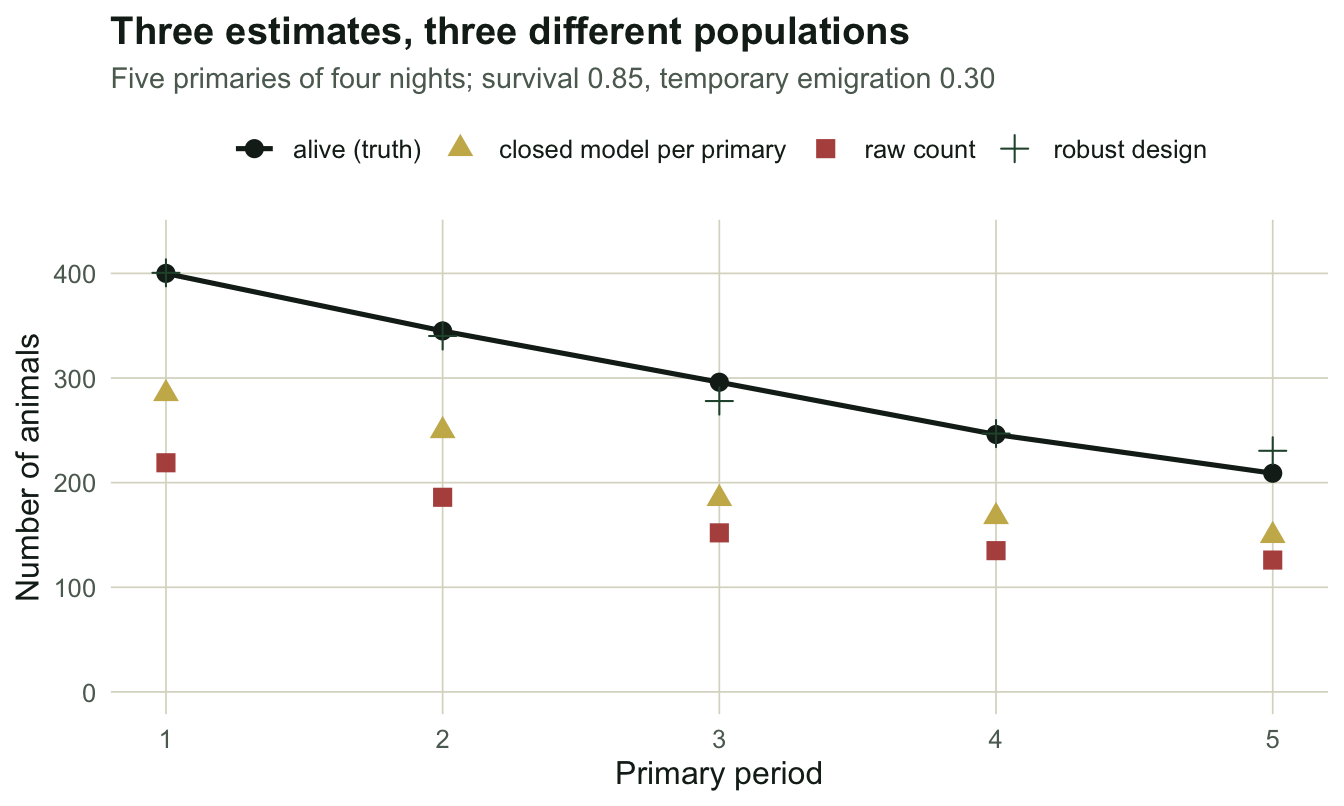
Is it consistent, or did we get lucky?
One dataset again. This world is small enough to check exactly: five primaries with counts in 0:4 give 3125 possible rows, and each has a closed-form probability under the forward algorithm. Weight every row by its exact probability, fit the model to those weights, and the answer is the probability limit.
all_rows <- function(Tp, K) as.matrix(expand.grid(rep(list(0:K), Tp))[, Tp:1])
rd_pd <- function(U, phi, g_io, g_oo, p, K, g_init) {
  Tm <- matrix(c(phi * (1 - g_io), phi * g_io, 1 - phi,
                 phi * (1 - g_oo), phi * g_oo, 1 - phi, 0, 0, 1), 3, 3, byrow = TRUE)
  E1 <- dbinom(0:K, K, p); d0 <- c(1 - g_init, g_init, 0)
  z <- (U == 0) * 1; out <- numeric(nrow(U))
  for (i in seq_len(nrow(U))) {
    al <- d0 * c(E1[U[i, 1] + 1], z[i, 1], z[i, 1])
    for (t in 2:ncol(U)) al <- as.vector(al %*% Tm) * c(E1[U[i, t] + 1], z[i, t], z[i, t])
    out[i] <- sum(al)
  }
  out
}
U   <- all_rows(Tp, K)
pdA <- rd_pd(U, phi, gam, gam, p, K, g_init = gam)
mass <- sum(pdA) - 1
kp  <- rowSums(U) > 0 & pdA > 1e-13
fr  <- 1e6 * pdA[kp] / sum(pdA[kp])
ex  <- fit_rd(U[kp, , drop = FALSE], K, markov = FALSE, wt = fr)
c(phi = ex$phi - phi, gamma = ex$g_io - gam, p = ex$p - p)
phi gamma p
1.470986e-08 -5.432028e-08 -1.795699e-08 The 3125 row probabilities sum to one up to floating-point rounding, which says the algebra is right. Fitted to those exact weights, the model returns survival off by \(1.47 \times 10^{-8}\), temporary emigration off by \(-5.43 \times 10^{-8}\), and capture off by \(-1.80 \times 10^{-8}\). That is optimiser tolerance. The estimator is consistent, and the three-way split is real and not a numerical accident.
Random or Markovian: the assumption inside the assumption
There are two ways to be away. Under random temporary emigration, every living animal tosses the same coin each period, whatever it did last time. Under Markovian emigration, animals that were away tend to stay away: absence has memory, which is what you expect from a breeding cycle or a foraging area an animal has settled into.
That distinction has no place in a CJS model, and it decides whether the survival estimate is fine or badly wrong.
all_hist <- function(k) as.matrix(expand.grid(rep(list(0:1), k))[, k:1])
rd_ph <- function(A, phi, g_io, g_oo, ps, g_init) {
  Tm <- matrix(c(phi * (1 - g_io), phi * g_io, 1 - phi,
                 phi * (1 - g_oo), phi * g_oo, 1 - phi, 0, 0, 1), 3, 3, byrow = TRUE)
  d0 <- c(1 - g_init, g_init, 0); out <- numeric(nrow(A))
  for (i in seq_len(nrow(A))) {
    em <- function(t, s) if (s == 1) (if (A[i, t] == 1) ps else 1 - ps) else as.numeric(A[i, t] == 0)
    al <- d0 * c(em(1, 1), em(1, 2), em(1, 3))
    for (t in 2:ncol(A)) al <- as.vector(al %*% Tm) * c(em(t, 1), em(t, 2), em(t, 3))
    out[i] <- sum(al)
  }
  out
}
A    <- all_hist(Tp)
g_oo <- 0.72                      # away animals stay away
g_st <- gam / (1 - g_oo + gam)    # stationary fraction away
cjs_rand <- fit_cjs(A, 1e6 * rd_ph(A, phi, gam, gam,  pin, g_init = gam))
cjs_mark <- fit_cjs(A, 1e6 * rd_ph(A, phi, gam, g_oo, pin, g_init = g_st))
c(random = cjs_rand$phi, markovian = cjs_mark$phi, truth = phi)
random markovian truth
0.8500000 0.7554723 0.8500000 Under random emigration the naive CJS converges to 0.850000, an error of \(-7.70 \times 10^{-7}\)%. This is the result that surprises people: ignore temporary emigration entirely, and if it is random, your survival estimate is still exactly right. Random absence is indistinguishable from a lower detection probability, and CJS was always going to report the product anyway.
Under Markovian emigration the same fit converges to 0.755472, an error of -11.12%. Memory in the absence process makes the gaps in a capture history longer than any constant detection can explain, and the likelihood has exactly one parameter that can lengthen gaps: mortality.
The robust design does not fix this by being a robust design. It fixes it by having the right transition matrix, and you have to ask for it.
pdM <- rd_pd(U, phi, gam, g_oo, p, K, g_init = g_st)
kpM <- rowSums(U) > 0 & pdM > 1e-13
frM <- 1e6 * pdM[kpM] / sum(pdM[kpM]); UM <- U[kpM, , drop = FALSE]
rd_wrong <- fit_rd(UM, K, markov = FALSE, wt = frM)
rd_right <- fit_rd(UM, K, markov = TRUE,  wt = frM)
c(rd_random = rd_wrong$phi, rd_markov = rd_right$phi, naive_cjs = cjs_mark$phi)
rd_random rd_markov naive_cjs
0.7554724 0.8500004 0.7554723 In the Markovian world, the robust design fitted with the random assumption converges to 0.755472, an error of -11.12%. That is 0.755472 for the naive CJS, and 0.755472 for the robust design: the same number. All the extra data bought nothing, because the mis-specification was in the state process, not in the detection model. Fitted with the Markovian transition, the same data give survival 0.850000 and both emigration parameters back: 0.300000 against a true 0.30, and 0.720001 against a true 0.72.
The honest limit: what absorbs the damage
Here is the awkward part. The robust design separates absence from detection by reading the zeros: an animal caught on night 1 and never again inside a period is evidence about p; a period with no captures at all is evidence about gamma. That reasoning assumes every present animal has the same p.
Suppose it does not. Half the animals are hard to catch (p = 0.15) and half are easy (p = 0.49). The mean is 0.32, exactly what it was before. Survival, emigration, everything else: unchanged. Only the constancy of p is broken, and it is broken in the least dramatic way available.
rd_pd_mix <- function(U, phi, g_io, g_oo, pv, wv, K, g_init) {
  o <- numeric(nrow(U))
  for (m in seq_along(pv)) o <- o + wv[m] * rd_pd(U, phi, g_io, g_oo, pv[m], K, g_init)
  o
}
pv <- c(0.15, 0.49); wv <- c(0.5, 0.5)
pdB <- rd_pd_mix(U, phi, gam, gam, pv, wv, K, g_init = gam)
kpB <- rowSums(U) > 0 & pdB > 1e-13
frB <- 1e6 * pdB[kpB] / sum(pdB[kpB])
het <- fit_rd(U[kpB, , drop = FALSE], K, markov = FALSE, wt = frB)

p_true_in <- sum(wv * (1 - (1 - pv)^K))   # true chance of catching a present animal
p_fit_in  <- 1 - (1 - het$p)^K            # what the fitted model believes
n_ratio   <- ((1 - gam) * p_true_in) / ((1 - het$g_io) * p_fit_in)
round(c(phi = het$phi, gamma = het$g_io, p = het$p), 4)
phi gamma p
0.8270 0.3556 0.3916 Survival is off by -2.70%, which is small. Temporary emigration comes back at 0.3556 against a true 0.30: an error of +18.54%.
Follow the mechanism. A present-but-shy animal produces a period of four zeros. The model has two explanations for four zeros, and only one of them is in its vocabulary for this animal: it was away. So the shy animals’ silent periods are booked as absence, gamma inflates, and the capture probability rises to 0.3916 to fit the animals that are left. The model now believes a present animal is caught with probability 0.8630 per period, when the truth is 0.7052. Abundance inherits both errors and lands at 0.8876 of the truth, or -11.24%.
The parameter that absorbs the damage is the one the design was built to estimate. That is worth sitting with: the robust design’s answer to “is it dead or elsewhere?” is only as good as its answer to “or is it just shy?”, and nothing in the fit complains.
The other honest limit: consistency is not usability
The Markovian model is the right one when absence has memory, and we showed above that it is consistent. Consistent means it converges as the data grow without bound. It does not mean it works on your study.
Nseq <- c(400, 800, 1600, 3200, 6400)
sw <- t(sapply(Nseq, function(NN) {
  PH <- NM <- numeric(100)
  for (b in 1:100) {
    ww <- sim_rd(NN, Tp, K, phi, gam, g_oo, p, seed = 70000 + b, g_init = g_st)
    DD <- ww$D[rowSums(ww$D) > 0, , drop = FALSE]
    f <- fit_rd(DD, K, markov = TRUE)
    PH[b] <- f$phi; NM[b] <- nrow(DD)
  }
  c(N = NN, marked = mean(NM), rmse = sqrt(mean((PH - phi)^2)), boundary = mean(PH > 0.99))
}))
round(sw, 4)
N marked rmse boundary
[1,] 400 275.97 0.0876 0.17
[2,] 800 552.77 0.0738 0.09
[3,] 1600 1108.61 0.0546 0.02
[4,] 3200 2215.77 0.0366 0.00
[5,] 6400 4423.67 0.0242 0.00At 276 marked animals over the same five primaries, which is a serious field season, the root mean squared error of survival is 0.0876 and 17 per cent of datasets run all the way to the boundary and report that nothing ever dies. You need 1109 marked animals before that drops to 2 per cent, and 4424 before the error is 0.0242.
df_sw <- data.frame(marked = sw[, "marked"], rmse = sw[, "rmse"],
                    lab = sprintf("%.0f%% at the boundary", 100 * sw[, "boundary"]))
ggplot(df_sw, aes(marked, rmse)) +
  geom_line(colour = te_forest, linewidth = 0.9) +
  geom_point(colour = te_forest, size = 3) +
  geom_text(aes(label = lab), vjust = c(-1.1, -1.1, -1.1, -1.1, 2),
            hjust = c(0, 0, 0, 0, 1),
            size = 3.4, colour = te_muted) +
  scale_x_log10(breaks = round(sw[, "marked"])) +
  scale_y_continuous(limits = c(0, 0.115)) +
  labs(title = "Consistent, and still not usable",
       subtitle = "Markovian robust design; 100 studies per size, true survival 0.85",
       x = "Marked animals (log scale)", y = "Survival RMSE") +
  theme_te()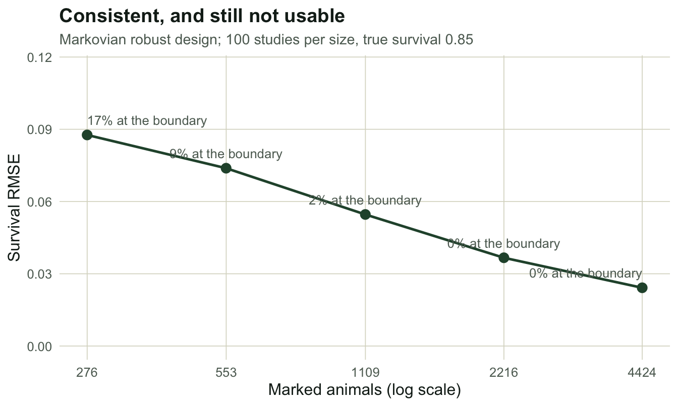
Both facts are true at once: the estimator is correct in the limit, and at the smallest study size simulated, a serious field season over five primary periods, about one dataset in six will tell you that survival is one. Consistency is a promise about a sequence of studies you will never do.
What to take away
The robust design is a design, and that is the point of it. The extra information does not come from a cleverer likelihood; it comes from sampling twice on two timescales, which is a decision you make in the field, before any of this code exists. Given that data, the three-state model separates dead from elsewhere from undetected, and it is consistent.
Then read the small print. Which kind of absence you assume decides whether survival is exact or eleven per cent low, and the data will not volunteer the answer. Heterogeneous detection is booked as temporary emigration, inflating the very parameter the design was built for. And with five primary periods, as in the sweep, the model that handles memory needs more animals than most studies will ever mark.
Checking an open-population model closes the series by asking what a goodness-of-fit test can see of any of this. Less than you would hope: the tests are computed on the marked animals, and most of these failures live in the animals nobody caught.
References
Pollock KH 1982 Journal of Wildlife Management 46:752-757 (10.2307/3808568)
Kendall WL, Nichols JD, Hines JE 1997 Ecology 78:563-578 (10.1890/0012-9658(1997)078[0563:ETEUCR]2.0.CO;2)
Kendall WL, Pollock KH, Brownie C 1995 Biometrics 51:293-308 (10.2307/2533335)
Pollock KH, Nichols JD, Brownie C, Hines JE 1990 Wildlife Monographs 107:1-97
Kendall WL 1999 Ecology 80:2517-2525 (10.1890/0012-9658(1999)080[2517:ROCCRM]2.0.CO;2)