library(ggplot2)

te_ink <- "#16241d"; te_forest <- "#275139"; te_gold <- "#c9b458"
te_rust <- "#b5534e"; te_sage <- "#93a87f"; te_line <- "#dad9ca"; te_muted <- "#5d6b61"

theme_te <- function() {
  theme_minimal(base_size = 12) +
    theme(
          plot.background  = element_rect(fill = "#f5f4ee", colour = NA),
          panel.background = element_rect(fill = "#f5f4ee", colour = NA),
          text = element_text(colour = te_ink),
          plot.title = element_text(face = "bold", colour = te_ink),
          plot.subtitle = element_text(colour = te_muted, size = rel(0.9)),
          axis.text = element_text(colour = te_muted),
          panel.grid.major = element_line(colour = te_line, linewidth = 0.3),
          panel.grid.minor = element_blank(),
          legend.position = "top", legend.title = element_blank())
}Pradel seniority: growth rate from reverse time
R
capture-recapture
population growth
population ecology
ecology tutorial
Run the same CJS likelihood on reversed capture histories to get seniority, turn it into a population growth rate, and see why its standard error lies.
Corrected 15 October 2026: the post said the bootstrap gets the width right and that its spread matches the Monte Carlo spread; it now says the bootstrap comes close, erring a little on the wide side, as its coverage run also shows.
Corrected 7 October 2026: the take-away called the direction of the delta-method error the flattering one; it now calls it the conservative one, as the coverage section shows.
Corrected 30 September 2026: the post stated the growth-rate and abundance errors as those of any study with a trap response; they belong to the one trap response simulated here, and the text now says so.
Forward in time, the Cormack-Jolly-Seber model asks: given that an animal is alive at occasion t, is it still alive at t + 1? The answer is apparent survival.
Run the film backwards and the same question becomes: given that an animal is alive at t, was it already there at t - 1? The answer is seniority, and Pradel (1996) showed that it is worth as much as survival, because the two together give you the population growth rate without ever counting anybody.
A population that grows
Seven occasions, survival 0.75, capture probability 0.32, and a population that starts at 150 animals and grows by 10 per cent per occasion. Those numbers fix the entries. If the population is N_t at occasion t and grows to N_t * lambda, then survival delivers N_t * phi of them and the rest have to arrive from somewhere: B_t = N_t * (lambda - phi) animals enter. Write that out and the entry probabilities are not a free parameter, they are arithmetic.
k <- 7; N1 <- 150; phi <- 0.75; lam <- 1.10; p <- 0.32
gam_true <- phi / lam
Bt   <- N1 * lam^(0:(k - 2)) * (lam - phi)
beta <- c(N1, Bt) / (N1 + sum(Bt))
Nsup <- round(N1 + sum(Bt))
c(sum_beta = sum(beta), superpop = Nsup)
sum_beta superpop
1 555 The superpopulation is 555 animals and the entry probabilities sum to 1. Seniority is the probability that an animal alive at t was already alive at t - 1, which under this bookkeeping is phi / lambda = 0.681818. That is the number we are trying to recover, and note what it is made of: it is a ratio of survival to growth, so the growth rate can be read back off it as phi divided by seniority.
sim_js <- function(N, beta, phi, p, seed, pf = p) {
  set.seed(seed); k <- length(beta)
  e <- sample.int(k, N, replace = TRUE, prob = beta)
  Alive <- matrix(FALSE, N, k)
  Alive[cbind(seq_len(N), e)] <- TRUE
  for (t in 2:k) Alive[, t] <- Alive[, t] | (Alive[, t - 1] & runif(N) < phi)
  H <- matrix(0L, N, k); seen <- rep(FALSE, N)
  for (t in seq_len(k)) {
    H[, t] <- as.integer(Alive[, t] & runif(N) < ifelse(seen, p, pf))
    seen <- seen | H[, t] == 1L
  }
  list(H = H, Alive = Alive)
}
d <- sim_js(Nsup, beta, phi, p, seed = 4277)
H <- d$H[rowSums(d$H) > 0, , drop = FALSE]
Nt_real <- colSums(d$Alive)
The realised population sizes are 167, 172, 186, 195, 200, 222, 252, so this run of the world grew from 167 to 252, and 305 animals were caught at least once.
The same code, backwards
Here is the CJS likelihood from the previous post, unchanged. It needs the occasion of first capture f, the occasion of last capture l, and the number of captures s; everything after l is absorbed by chi.
hsum <- function(H) {
  k <- ncol(H); idx <- col(H) * H; idx[idx == 0] <- NA
  list(f = suppressWarnings(apply(idx, 1, min, na.rm = TRUE)),
       l = suppressWarnings(apply(idx, 1, max, na.rm = TRUE)),
       s = rowSums(H), k = k)
}
chi_vec <- function(phi, p, k) {
  chi <- numeric(k); chi[k] <- 1
  for (j in (k - 1):1) chi[j] <- (1 - phi) + phi * (1 - p) * chi[j + 1]
  chi
}
cjs_nll <- function(par, S) {
  phi <- plogis(par[1]); p <- plogis(par[2]); chi <- chi_vec(phi, p, S$k)
  v <- -sum(log(phi^(S$l - S$f) * p^(S$s - 1) * (1 - p)^(S$l - S$f - S$s + 1) * chi[S$l]))
  if (!is.finite(v)) 1e10 else v
}
fit_cjs <- function(H) {
  S <- hsum(H[rowSums(H) > 0, , drop = FALSE])
  fit <- optim(c(qlogis(0.7), qlogis(0.3)), cjs_nll, S = S, method = "BFGS", hessian = TRUE)
  V <- tryCatch(solve(fit$hessian), error = function(e) matrix(NA, 2, 2))
  se <- sqrt(diag(V)); ph <- plogis(fit$par[1]); pd <- plogis(fit$par[2])
  list(phi = ph, p = pd, se_phi = se[1] * ph * (1 - ph), se_p = se[2] * pd * (1 - pd))
}
Now the whole trick. Reverse the columns of the capture matrix and fit again.
fwd <- fit_cjs(H)
rev <- fit_cjs(H[, k:1])
lam_hat <- fwd$phi / rev$phi
Forward, the model returns apparent survival 0.7723 (SE 0.0311) against a true 0.75. Backwards, the identical function returns 0.7259 (SE 0.0298) against a true seniority of 0.6818. Nothing in the code knows which way time runs. The reversed data has first captures where the last captures were, and the parameter the likelihood calls survival is now the probability of having been there already.
Divide one by the other and the growth rate falls out:
c(lambda_hat = lam_hat, truth = lam)lambda_hat truth
1.063935 1.100000 1.0639 against a true 1.10, from a dataset in which nobody was counted. The population size never appears. Both fits condition on first capture, so the animals nobody ever caught are as irrelevant here as they are to survival.
Is the identity real, or is this a coincidence?
One dataset proves nothing, and lambda = phi / gamma looks suspiciously tidy. Take the sampling noise out: enumerate all 128 possible capture histories, weight each by its exact probability under the true world, and fit the two models to the expected frequencies. What comes back is the probability limit.
all_hist <- function(k) as.matrix(expand.grid(rep(list(0:1), k))[, k:1])
popan_ph2 <- function(S, phi, pf, p, beta) {
  k <- S$k
  chi <- chi_vec(phi, p, k)
  nu <- numeric(k); nu[k] <- 1 - pf
  for (e in (k - 1):1) nu[e] <- (1 - pf) * ((1 - phi) + phi * nu[e + 1])
  x <- phi * (1 - pf); g <- numeric(k); g[1] <- beta[1]
  for (f in 2:k) g[f] <- x * g[f - 1] + beta[f]
  out <- numeric(length(S$s)); out[S$s == 0] <- sum(beta * nu)
  ok <- S$s > 0; f <- S$f[ok]; l <- S$l[ok]; s <- S$s[ok]
  out[ok] <- g[f] * pf * phi^(l - f) * p^(s - 1) * (1 - p)^(l - f - s + 1) * chi[l]
  out
}
cjs_nll_f <- function(par, S, fr) {
  phi <- plogis(par[1]); p <- plogis(par[2]); chi <- chi_vec(phi, p, S$k)
  v <- -sum(fr * log(phi^(S$l - S$f) * p^(S$s - 1) * (1 - p)^(S$l - S$f - S$s + 1) * chi[S$l]))
  if (!is.finite(v)) 1e10 else v
}
fit_cjs_f <- function(A, fr) {
  ok <- rowSums(A) > 0; S <- hsum(A[ok, , drop = FALSE])
  f <- optim(c(qlogis(.7), qlogis(.3)), cjs_nll_f, S = S, fr = fr[ok], method = "BFGS",
             control = list(reltol = 1e-14, maxit = 5000))
  list(phi = plogis(f$par[1]), p = plogis(f$par[2]))
}

A  <- all_hist(k);   S  <- hsum(A)
Ar <- A[, k:1];      Sr <- hsum(Ar)
M  <- 1e6
ph <- popan_ph2(S, phi, p, p, beta); fr <- M * ph
ex_f <- fit_cjs_f(A[S$s > 0, , drop = FALSE], fr[S$s > 0])
ex_r <- fit_cjs_f(Ar[Sr$s > 0, , drop = FALSE], fr[Sr$s > 0])
gap  <- ex_r$phi - gam_true
With infinite data the forward fit converges to 0.75000003 and the reverse fit to 0.68181820, against a seniority of 0.68181818. The difference is \(2.286 \times 10^{-8}\), which is optimiser tolerance rather than bias, and the implied growth rate is 1.10000001. The identity is exact. Reverse-time seniority is not an approximation or a rule of thumb: it is what the reversed likelihood is consistent for.
Three questions, one dataset, three levels of exposure
Both fits condition on first capture, so neither of them models it. That is the protection, and the previous post showed what happens to a model that gives the protection up: POPAN buys abundance by assuming the first capture works like a recapture, and collapses when it does not.
So put all three questions in the same broken world. Animals that have never been handled are caught with probability 0.18; once marked, 0.45. Everything else is as before, and everything is computed exactly, with no sampling noise anywhere.
nu_vec <- function(phi, p, k) {
  nu <- numeric(k); nu[k] <- 1 - p
  for (e in (k - 1):1) nu[e] <- (1 - p) * ((1 - phi) + phi * nu[e + 1])
  nu
}
ent_vec <- function(phi, p, beta, k) {
  x <- phi * (1 - p); g <- numeric(k); g[1] <- beta[1]
  for (f in 2:k) g[f] <- x * g[f - 1] + beta[f]
  g
}
popan_ph <- function(S, phi, p, beta) {
  k <- S$k; chi <- chi_vec(phi, p, k); g <- ent_vec(phi, p, beta, k)
  ok <- S$s > 0; out <- numeric(length(S$s))
  out[!ok] <- sum(beta * nu_vec(phi, p, k))
  f <- S$f[ok]; l <- S$l[ok]; s <- S$s[ok]
  out[ok] <- g[f] * p * phi^(l - f) * p^(s - 1) * (1 - p)^(l - f - s + 1) * chi[l]
  out
}
popan_nll <- function(par, freq, S, n) {
  k <- S$k
  N <- n + exp(par[1]); phi <- plogis(par[2]); p <- plogis(par[3])
  bl <- c(0, par[4:(k + 2)]); beta <- exp(bl) / sum(exp(bl))
  ph <- popan_ph(S, phi, p, beta)
  P0 <- ph[S$s == 0]
  if (!is.finite(P0) || P0 <= 0 || P0 >= 1) return(1e10)
  pv <- ph[S$s > 0]; if (any(!is.finite(pv)) || any(pv <= 0)) return(1e10)
  v <- -(lgamma(N + 1) - lgamma(N - n + 1) + (N - n) * log(P0) + sum(freq * log(pv)))
  if (!is.finite(v)) 1e10 else v
}
fit_popan_f <- function(A, fr, n) {
  S <- hsum(A); k <- S$k
  f <- optim(c(log(0.5 * n), qlogis(.7), qlogis(.3), rep(0, k - 1)), popan_nll,
             freq = fr[S$s > 0], S = S, n = n, method = "BFGS",
             control = list(reltol = 1e-14, maxit = 8000))
  n + exp(f$par[1])
}

pht  <- popan_ph2(S, phi, 0.18, 0.45, beta); frt <- M * pht
tr_f <- fit_cjs_f(A[S$s > 0, , drop = FALSE], frt[S$s > 0])
tr_r <- fit_cjs_f(Ar[Sr$s > 0, , drop = FALSE], frt[Sr$s > 0])
tr_N <- fit_popan_f(A, frt, M * (1 - pht[S$s == 0]))
err  <- c(phi    = 100 * (tr_f$phi / phi - 1),
          gamma  = 100 * (tr_r$phi / gam_true - 1),
          lambda = 100 * ((tr_f$phi / tr_r$phi) / lam - 1),
          N      = 100 * (tr_N / M - 1))
round(err, 2)
phi gamma lambda N
0.00 -3.87 4.03 -46.32 fmt_pct <- function(x) ifelse(abs(x) < 0.005, "0.00%", sprintf("%+.2f%%", x))Survival is untouched: 0.00%. Seniority moves by -3.87% and the growth rate by +4.03%. The superpopulation is out by -46.32%.
lab <- c(phi = "survival", gamma = "seniority", lambda = "growth rate",
         N = "superpopulation")
df_g <- data.frame(what = factor(lab[names(err)], levels = lab),
                   err = as.numeric(err),
                   band = c("conditions on first capture", "conditions on first capture",
                            "conditions on first capture", "models first capture"))
p_grad <- ggplot(df_g, aes(what, err, fill = band)) +
  geom_col(width = 0.62) +
  geom_hline(yintercept = 0, colour = te_ink, linewidth = 0.5) +
  geom_text(aes(label = fmt_pct(err),
                vjust = ifelse(err < 0, 1.5, -0.6)), size = 3.6, colour = te_ink) +
  scale_fill_manual(values = c(`conditions on first capture` = te_forest,
                               `models first capture` = te_rust)) +
  scale_y_continuous(limits = c(-58, 14)) +
  labs(title = "The same assumption, three levels of exposure",
       subtitle = "Exact asymptotic error, naive capture 0.18 against recapture 0.45",
       x = NULL, y = "Error in the probability limit") +
  theme_te()
p_grad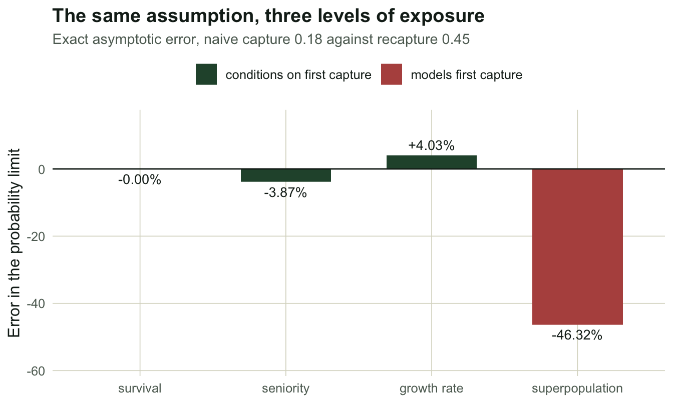
The gradient is not luck. Survival is protected because the likelihood conditions on first capture, so pf never enters it. Seniority is estimated by the same conditioning, but on reversed data, where the last capture is what gets conditioned on and the first capture is one of the events being modelled: the protection is partial. And the growth rate is a ratio of the two, so it inherits whatever seniority inherits. POPAN, which needs the first capture to build a superpopulation, gets the whole of it.
In this scenario, where marking more than doubles the capture probability, the growth rate comes out about four per cent wrong and the abundance nearly half wrong; a weaker or stronger trap response moves both numbers. The same data, the same assumption, the same violation.
The standard error is not honest
Here is a subtler failure, and it has nothing to do with trap response. Go back to the model-true world, simulate 200 fresh studies, and compare the delta-method standard error for lambda with the actual spread of lambda.
LA <- SE <- numeric(200)
for (b in 1:200) {
  dd <- sim_js(Nsup, beta, phi, p, seed = 40000 + b)
  Hb <- dd$H[rowSums(dd$H) > 0, , drop = FALSE]
  f <- fit_cjs(Hb); r <- fit_cjs(Hb[, k:1])
  LA[b] <- f$phi / r$phi
  SE[b] <- LA[b] * sqrt((f$se_phi / f$phi)^2 + (r$se_phi / r$phi)^2)
}
mc_sd <- sd(LA); mean_se <- mean(SE)
The estimator itself is fine: mean 1.0993 against a true 1.10, a bias of -0.0007. But the spread of those 200 estimates is 0.0242, and the average delta-method standard error is 0.0734. The reported uncertainty is 3.0 times too wide.
The delta method is not broken; it was given a false premise. The usual formula for the standard error of a ratio treats the numerator and the denominator as independent. Here they come from the same animals: a study that happens to contain long-lived individuals returns a high phi and a high gamma together, and the ratio is steadier than either part. Adding the two relative variances counts a cancellation as if it were noise.
Bootstrap the whole procedure
The fix is to resample what was actually random, which is the animals, and then repeat both fits on each replicate. Whatever correlation the two estimates have, the bootstrap reproduces it, because it never has to know it exists.
fit_cjs_ph <- function(H) {
  S <- hsum(H[rowSums(H) > 0, , drop = FALSE])
  o <- optim(c(qlogis(0.7), qlogis(0.3)), cjs_nll, S = S, method = "BFGS")
  plogis(o$par[1])
}
boot_lambda <- function(H, B, seed) {
  set.seed(seed); n <- nrow(H); kk <- ncol(H); out <- numeric(B)
  for (b in seq_len(B)) {
    Hb <- H[sample.int(n, n, replace = TRUE), , drop = FALSE]
    out[b] <- tryCatch(fit_cjs_ph(Hb) / fit_cjs_ph(Hb[, kk:1]), error = function(e) NA_real_)
  }
  out[is.finite(out)]
}
bl  <- boot_lambda(H, B = 500, seed = 5277)
qb  <- quantile(bl, c(0.025, 0.975))
del <- lam_hat * sqrt((fwd$se_phi / fwd$phi)^2 + (rev$se_phi / rev$phi)^2)
wald <- c(lam_hat - 1.96 * del, lam_hat + 1.96 * del)
The bootstrap standard deviation is 0.0261. The Monte Carlo spread, which is the truth, was 0.0242. The bootstrap comes close to the right width from a single dataset, erring a little on the wide side, without being told anything about the correlation it is correcting for.
The percentile interval is [1.0164, 1.1164], a width of 0.1000. The Wald interval is [0.9440, 1.1839], a width of 0.2398, or 2.4 times wider.
df_b  <- data.frame(lam = bl)
df_ci <- data.frame(
  kind = c("percentile (bootstrap)", "Wald (delta method)"),
  lo   = c(qb[1], wald[1]), hi = c(qb[2], wald[2]), y = c(78, 88))
ggplot(df_b, aes(lam)) +
  geom_histogram(bins = 32, fill = te_forest, alpha = 0.8, colour = NA) +
  geom_vline(xintercept = lam, colour = te_ink, linetype = 2, linewidth = 0.8) +
  geom_errorbar(data = df_ci, aes(xmin = lo, xmax = hi, y = y, colour = kind),
                inherit.aes = FALSE, orientation = "y", width = 6, linewidth = 1.1) +
  annotate("text", x = lam + 0.004, y = 60, label = "truth", colour = te_ink,
           hjust = 0, size = 3.6, fontface = "bold") +
  scale_colour_manual(values = c(`percentile (bootstrap)` = te_gold,
                                 `Wald (delta method)` = te_rust)) +
  labs(title = "One dataset, two accounts of the same uncertainty",
       subtitle = sprintf("500 replicates; bootstrap SD %.4f against a Monte Carlo spread of %.4f",
                          sd(bl), mc_sd),
       x = "Population growth rate", y = "Bootstrap replicates") +
  theme_te()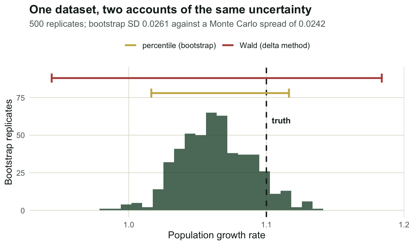
Width is not the point, though. Coverage is. Run both intervals over 200 fresh studies and ask how often each one contains the true 1.10.
cvB <- cvD <- wB <- wD <- numeric(200)
for (b in 1:200) {
  dd <- sim_js(Nsup, beta, phi, p, seed = 40000 + b)
  Hb <- dd$H[rowSums(dd$H) > 0, , drop = FALSE]
  f <- fit_cjs(Hb); r <- fit_cjs(Hb[, k:1]); L <- f$phi / r$phi
  s <- L * sqrt((f$se_phi / f$phi)^2 + (r$se_phi / r$phi)^2)
  cvD[b] <- abs(L - lam) < 1.96 * s; wD[b] <- 2 * 1.96 * s
  qq <- quantile(boot_lambda(Hb, B = 200, seed = 90000 + b), c(0.025, 0.975))
  cvB[b] <- qq[1] <= lam && lam <= qq[2]; wB[b] <- diff(qq)
}
The bootstrap interval covers 98.5% of the time with a mean width of 0.1037. The Wald interval covers 100.0% of the time with a mean width of 0.2879.
Read the second one again. The delta-method interval is not anticonservative here: it is not lying about the parameter, it is refusing to say anything. Covering 100 per cent of the time is not a 95 per cent interval; it is an interval that has given up. The failure is easy to miss precisely because it points the safe way, and a reviewer who checks that your interval is not too narrow will never catch it.
What to take away
Reverse-time seniority is one of the best deals in capture-recapture: no new model, no new data, no counting, and the growth rate comes out of code you already have. Pay attention to two things.
The first is what the estimate is exposed to. Survival, seniority and abundance sit at increasing distances from the first capture, and their errors under the same violation are ordered the same way. The second is that a quantity built from two fits needs an uncertainty built the same way. The delta method assumed independence that was not there, and the direction of that error is the conservative one, which is why it is easy to miss.
The robust design post goes after the information that would settle the first capture question by changing the field protocol rather than the likelihood. And checking an open-population model asks whether a goodness-of-fit test would have told you any of this. It would not.
References
Pradel 1996 Biometrics 52:703-709 (10.2307/2532908)
Schwarz & Arnason 1996 Biometrics 52:860-873 (10.2307/2533048)
Jolly 1965 Biometrika 52(1-2):225-248 (10.1093/biomet/52.1-2.225)
Efron & Tibshirani 1993 An Introduction to the Bootstrap, Chapman & Hall (ISBN 978-0-412-04231-7)
Link 2003 Biometrics 59(4):1123-1130 (10.1111/j.0006-341X.2003.00129.x)